Full detector response

The detector response provides us with the the following information:

• The effective area at a given energy for a given direction. This allows us to convert from counts to physical quantities like flux

• The expected distribution of measured energy and other reconstructed quantities. This allows us to account for all sorts of detector effects when we do our analysis.

This tutorial will show you how to handle the detector response and extract useful information from it.

Dependencies

%%capture
import numpy as np
import astropy.units as u
from astropy.units import Quantity
from astropy.coordinates import SkyCoord
from astropy.io import fits
from astropy.time import Time

import matplotlib.pyplot as plt
import matplotlib.pyplot as ply

from mhealpy import HealpixMap, HealpixBase
import pandas as pd
from pathlib import Path

from scoords import Attitude, SpacecraftFrame
from cosipy.response import FullDetectorResponse
from cosipy.spacecraftfile import SpacecraftHistory
from cosipy import test_data
from cosipy.util import fetch_wasabi_file
from histpy import Histogram
import gc

from threeML import Model, Powerlaw

from cosipy.response import FullDetectorResponse

import shutil
import os

File downloads

You can skip this step if you’ve already downloaded the files. Make sure that paths point to the right files

data_dir = Path("") # Current directory by default. Modify if you can want a different path

ori_path = data_dir/"20280301_3_month_with_orbital_info.fits"
response_path = data_dir/"SMEXv12.Continuum.HEALPixO3_10bins_log_flat.binnedimaging.imagingresponse.h5"

# download orientation file ~684.38 MB
fetch_wasabi_file("COSI-SMEX/develop/Data/Orientation/20280301_3_month_with_orbital_info.fits", ori_path, checksum = '5e69bc1d55fab9390f90635690f62896')

# download response file ~596.06 MB
fetch_wasabi_file("COSI-SMEX/develop/Data/Responses/SMEXv12.Continuum.HEALPixO3_10bins_log_flat.binnedimaging.imagingresponse.h5", checksum = 'eb72400a1279325e9404110f909c7785')

A file named 20280301_3_month_with_orbital_info.fits already exists with the specified checksum (5e69bc1d55fab9390f90635690f62896). Skipping.
A file named SMEXv12.Continuum.HEALPixO3_10bins_log_flat.binnedimaging.imagingresponse.h5 already exists with the specified checksum (eb72400a1279325e9404110f909c7785). Skipping.

Opening a full detector response

The response of the instrument in encoded in a series of matrices cointained in a file. You can open the file like this:

response = FullDetectorResponse.open(response_path)

print(response.filename)

response.close()

SMEXv12.Continuum.HEALPixO3_10bins_log_flat.binnedimaging.imagingresponse.h5

Or if you don’t want to worry about closing the file, use a context manager statement:

with FullDetectorResponse.open(response_path) as response:

    print(repr(response))

FILENAME: '/Users/imartin5/software/cosipy/docs/tutorials/response/SMEXv12.Continuum.HEALPixO3_10bins_log_flat.binnedimaging.imagingresponse.h5'
AXES:
  NuLambda:
    DESCRIPTION: 'Location of the simulated source in the spacecraft coordinates'
    TYPE: 'healpix'
    NPIX: 768
    NSIDE: 8
    SCHEME: 'RING'
  Ei:
    DESCRIPTION: 'Initial simulated energy'
    TYPE: 'log'
    UNIT: 'keV'
    NBINS: 10
    EDGES: [100.0 keV, 158.489 keV, 251.189 keV, 398.107 keV, 630.957 keV, 1000.0 keV, 1584.89 keV, 2511.89 keV, 3981.07 keV, 6309.57 keV, 10000.0 keV]
  Em:
    DESCRIPTION: 'Measured energy'
    TYPE: 'log'
    UNIT: 'keV'
    NBINS: 10
    EDGES: [100.0 keV, 158.489 keV, 251.189 keV, 398.107 keV, 630.957 keV, 1000.0 keV, 1584.89 keV, 2511.89 keV, 3981.07 keV, 6309.57 keV, 10000.0 keV]
  Phi:
    DESCRIPTION: 'Compton angle'
    TYPE: 'linear'
    UNIT: 'deg'
    NBINS: 36
    EDGES: [0.0 deg, 5.0 deg, 10.0 deg, 15.0 deg, 20.0 deg, 25.0 deg, 30.0 deg, 35.0 deg, 40.0 deg, 45.0 deg, 50.0 deg, 55.0 deg, 60.0 deg, 65.0 deg, 70.0 deg, 75.0 deg, 80.0 deg, 85.0 deg, 90.0 deg, 95.0 deg, 100.0 deg, 105.0 deg, 110.0 deg, 115.0 deg, 120.0 deg, 125.0 deg, 130.0 deg, 135.0 deg, 140.0 deg, 145.0 deg, 150.0 deg, 155.0 deg, 160.0 deg, 165.0 deg, 170.0 deg, 175.0 deg, 180.0 deg]
  PsiChi:
    DESCRIPTION: 'Location in the Compton Data Space'
    TYPE: 'healpix'
    NPIX: 768
    NSIDE: 8
    SCHEME: 'RING'

Although opening a detector response does not load the matrices, it loads all the header information above. This allows us to pass it around for various analysis at a very low cost.

Detector response matrix

The full –i.e. all-sky– detector response is encoded in a HEALPix grid. For each pixel there is a multidimensional matrix describing the response of the instrument for that particular direction in the spacefraft coordinates. For this response has the following grid:

with FullDetectorResponse.open(response_path) as response:

    print(f"NSIDE = {response.nside}")
    print(f"SCHEME = {response.scheme}")
    print(f"NPIX = {response.npix}")
    print(f"Pixel size = {np.sqrt(response.pixarea()).to(u.deg):.2f}")

NSIDE = 8
SCHEME = RING
NPIX = 768
Pixel size = 7.33 deg

To retrieve the detector response matrix for a given pixel simply use the [] operator

with FullDetectorResponse.open(response_path) as response:

    print(f"Pixel 0 centered at {response.pix2skycoord(0)}")
    drm = response[0]

Pixel 0 centered at <SkyCoord (SpacecraftFrame: attitude=None, obstime=None, location=None): (lon, lat) in deg
    (45., 84.14973294)>

Or better, get the interpolated matrix for a given direction. In this case, for the on-axis response:

with FullDetectorResponse.open(response_path) as response:

    drm = response.get_interp_response(SkyCoord(lon = 0*u.deg, lat = 90*u.deg, frame = SpacecraftFrame()))

The matrix has multiple dimensions, including real photon initial energy, the measured energy, the Compton data space, and possibly other:

drm.axes.labels

array(['Ei', 'Em', 'Phi', 'PsiChi'], dtype='<U6')

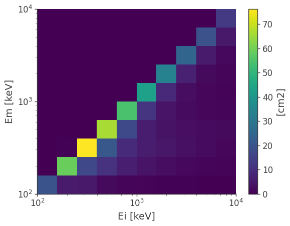
However, one of the most common operation is to get the effective area and the energy dispersion matrix. This is encoded in a reduced detector response, which is the projection of the full matrix into the initial and measured energy axes:

drm.get_spectral_response().plot();

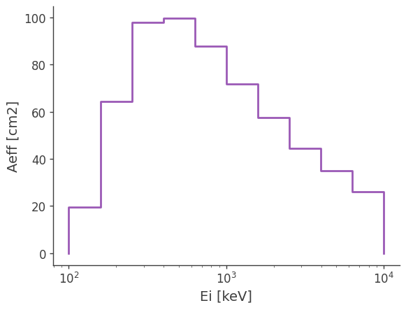
You can further project it into the initial energy to get the effective area:

ax,plot = drm.get_effective_area().plot();

ax.set_ylabel(f'Aeff [{drm.unit}]');

Get the interpolated effective area

drm.get_effective_area(511*u.keV)

$99.27511 \; \mathrm{cm^{2}}$

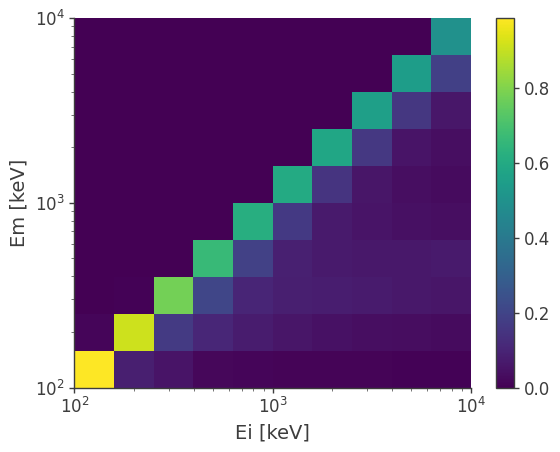
Or the energy dispersion matrix

drm.get_dispersion_matrix().plot();

Point source response and expected counts

Once we have the response, the next step is usually to get the expected counts for a specific source. However, it is not trivial for the case of a spacecraft because the response we have here is the detector response. This response records the detector effects to given points viewed from the reference frame attached to the spacecraft (SC).

A source with a fixed position on the sky is moving from the perspective of the spacecraft (detector). Therefore, we need to convert the coordinate of a source to the reference frame, which results in a moving point viewed from the spacecraft. By convolving the trajectory of the source in the spacecraft frame with the detector response, we will get the so-called point source response.

See the spacecraft file tutorial for a discussion of the SC attitude history, transformations to/from galactic coordinates, and the dwell time map.

# Read the full orientation
ori = SpacecraftHistory.open(ori_path)

# Define the target coordinates (Crab)
target_coord = SkyCoord(184.5551, -05.7877, unit = "deg", frame = "galactic")

# Get the dwell time map
with FullDetectorResponse.open(response_path) as response:
    dwell_time_map = ori.get_dwell_map(target_coord = target_coord, base = response)

We can now convolve the exposure map with the full detector response, and get a PointSourceResponse

with FullDetectorResponse.open(response_path) as response:
    psr = response.get_point_source_response(exposure_map = dwell_time_map, coord = target_coord)

Note that a PointSourceResponse only depends on the path of the source, not on the spectrum of the source. It has units of area*time

psr.unit

$\mathrm{cm^{2}\,s}$

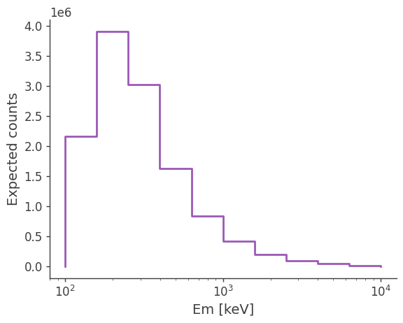
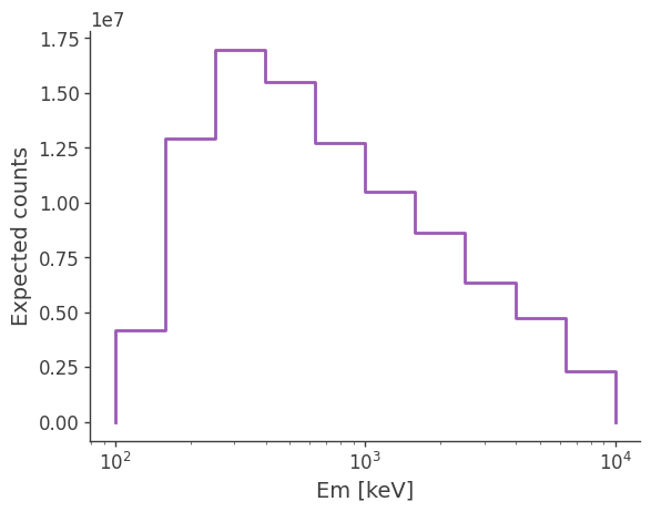
Finally, we convolve a spectrum to get the expected excess for each measured energy bin:

index = -2.2
K = 10**-3 / u.cm / u.cm / u.s / u.keV
piv = 100 * u.keV

spectrum = Powerlaw()
spectrum.index.value = index
spectrum.K.value = K.value
spectrum.piv.value = piv.value
spectrum.K.unit = K.unit
spectrum.piv.unit = piv.unit

expectation = psr.get_expectation(spectrum)

ax, plot = expectation.project('Em').plot()

ax.set_ylabel('Expected counts')

Text(0, 0.5, 'Expected counts')

Try changing the spectrum and see how the expected excess changes.

spectrum.index.value = -1

expectation = psr.get_expectation(spectrum)

ax, plot = expectation.project('Em').plot()

ax.set_ylabel('Expected counts')

Text(0, 0.5, 'Expected counts')

Point source response in inertial coordinates

In the previous example we obtained the response for a point source as seen in the reference frame attached to the spacecraft (SC) frame. As the spacecraft rotates, a fixed source in the sky is seen by the detector from multiple directions, so binning the data on the spacecraft coordinate, without binning it simultaneously in time, can wash out the signal. As shown in this section, we can instead rotate the response and convolve it with the attitude history of the spacecraft, resulting in a point source response with a Compton data space binned in inertial coordinates.

We use a scatt map, which tracks the amount of time the spacecraft spent in a given orientation. See spacecraft file tutorial for more details.

scatt_map = ori.get_scatt_map(nside = 16, earth_occ = False)

Now we can let cosipy perform the convolution with the scatt map and get the point source response:

%%time

from astropy.coordinates import SkyCoord

coord = SkyCoord.from_name('Crab').galactic

with FullDetectorResponse.open(response_path) as response:
    psr = response.get_point_source_response(coord = coord, scatt_map = scatt_map)

CPU times: user 2.04 s, sys: 38.7 ms, total: 2.08 s
Wall time: 2.08 s

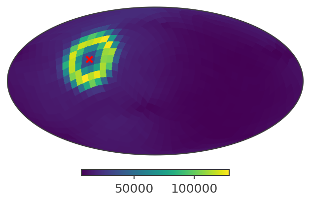
This is how a slice of the response looks like in galactic coordinates:

psichi_slice = psr.slice[{'Ei':4, 'Phi':4}].project('PsiChi')

ax,plot = psichi_slice.plot(ax_kw = {'coord':'G'})

ax.scatter([coord.l.deg], [coord.b.deg], transform = ax.get_transform('world'), marker = 'x', color = 'red')

<matplotlib.collections.PathCollection at 0x15796a4e0>

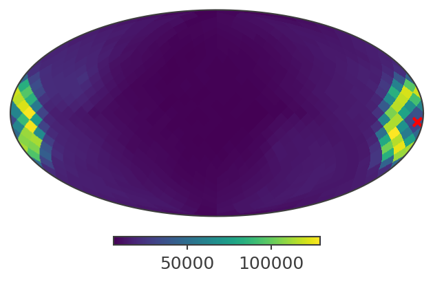
And here in ICRS (RA/Dec)

ax,plot = psichi_slice.plot(ax_kw = {'coord':'C'})

ax.scatter([coord.icrs.ra.deg], [coord.icrs.dec.deg], transform = ax.get_transform('world'), marker = 'x', color = 'red')

<matplotlib.collections.PathCollection at 0x168c9aa20>

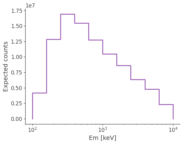
You can also use it the same way as a point source response obtained from a exposure map. e.g.

expectation = psr.get_expectation(spectrum)

ax, plot = expectation.project('Em').plot()

ax.set_ylabel('Expected counts')

Text(0, 0.5, 'Expected counts')

XSPEC support

You can also convert the point source response to XSPEC readable files (arf, rmf and pha) if you want to do spectral fitting or simulation in XSPEC.

Warning: RspArfRmfConverter currently only supports local spacecraft coordinate. Therefore, it is limited to short-duration events.

from cosipy.response import RspArfRmfConverter

response = FullDetectorResponse.open(response_path)
rsp_converter = RspArfRmfConverter(response, ori, coord)

Ei_edges, Ei_lo, Ei_hi, Em_edges, Em_lo, Em_hi, arf, rmf = rsp_converter.get_psr_rsp()

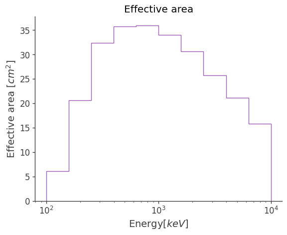
rsp_converter.write_arf("Crab.arf", overwrite = True)
rsp_converter.plot_arf()

<Axes: title={'center': 'Effective area'}, xlabel='Energy[$keV$]', ylabel='Effective area [$cm^2$]'>

rsp_converter.write_rmf("Crab.rmf", overwrite = True)
rsp_converter.plot_rmf()

---------------------------------------------------------------------------
TypeError                                 Traceback (most recent call last)
Cell In[31], line 2
      1 rsp_converter.write_rmf("Crab.rmf")
----> 2 rsp_converter.plot_rmf()

File ~/software/cosipy/cosipy/response/rsp_to_arf_rmf.py:465, in RspArfRmfConverter.plot_rmf(self, ax, file_name)
    463 matrix = data[i][5]  # get the probabilities of this row (incident energy)
    464 indices = []
--> 465 for k in f_chan:
    466     channels = np.arange(k, k + n_chan[np.argwhere(f_chan == k)][0][0]).tolist()  # generate the cha
    467     indices += channels  # append the channels together

TypeError: 'numpy.float32' object is not iterable