Diffuse 511 Spectral Fit in Galactic Coordinates
This notebook fits the spectrum for the 511 keV emission in the Galaxy. It can be used as a general template for fitting diffuse/extended sources in Galactic coordinates. For a general introduction into spectral fitting with cosipy, see the continuum_fit tutorial.
This notebook uses two 511 keV emission models, first a test model and then a realistic multi-component model.
All input models are available here: https://github.com/cositools/cosi-data-challenges/tree/main/cosi_dc/Source_Library/DC2/sources/511
The toy 511 model consists of two components: an extended Gaussian source (5 degree extension) and a point source. In the first part of this tutorial, we fit the data with just the single extended Gaussian component, i.e. we ignore the point source component. This is done as a simplification, and as will be seen, it already provides a good fit. In the second part of this tutorial we use a model consisting of both components.
The realistic input models consist of a bulge component (with an extended Gaussian source and a point source) as well as a disk component with different spectral characteristics. In the third part of this tutorial we use this model.
For the background we use just the cosmic photons.
This tutotrial also walks through all the steps needed when performing a spectral fit, starting with the unbinned data, i.e. creating the combined data set, and binning the data.
For the first two examples, you will need the following files (available on wasabi): 20280301_3_month_with_orbital_info.ori cosmic_photons_3months_unbinned_data.fits.gz 511_Testing_3months.fits.gz SMEXv12.511keV.HEALPixO4.binnedimaging.imagingresponse.h5 psr_gal_511_DC2.h5
The binned data products are available on wasabi, so you can also start by loading the binned data directly.
For the third example, we start with the binned data, and you will need: combined_binned_data_thin_disk.hdf5
WARNING: If you run into memory issues creating the combined dataset or binning the data on your own, start by just loading the binned data directly. See the dataIO example for how to deal with memory issues.
[1]:
import logging
import sys
import os


logger = logging.getLogger('cosipy')
logger.setLevel(logging.INFO)
logger.addHandler(logging.StreamHandler(sys.stdout))

os.environ["OMP_NUM_THREADS"] = "1"
os.environ["MKL_NUM_THREADS"] = "1"
os.environ["NUMEXPR_NUM_THREADS"] = "1"
[2]:
# imports:
from cosipy import test_data, BinnedData
from cosipy.spacecraftfile import SpacecraftHistory
from cosipy.response.FullDetectorResponse import FullDetectorResponse
from cosipy.response.ExtendedSourceResponse import ExtendedSourceResponse

from cosipy.util import fetch_wasabi_file

from cosipy.statistics import PoissonLikelihood
from cosipy.background_estimation import FreeNormBinnedBackground
from cosipy.interfaces import ThreeMLPluginInterface
from cosipy.response import BinnedThreeMLModelFolding, BinnedInstrumentResponse, BinnedThreeMLExtendedSourceResponse,BinnedThreeMLPointSourceResponse
from cosipy.data_io import EmCDSBinnedData


from scoords import SpacecraftFrame

from astropy.time import Time
import astropy.units as u
from astropy.coordinates import SkyCoord, Galactic

import numpy as np
import matplotlib.pyplot as plt

from threeML import  PointSource, Model, JointLikelihood, DataList, update_logging_level
from astromodels import Model, Parameter, PointSource, ExtendedSource, Gaussian, Gaussian_on_sphere, Asymm_Gaussian_on_sphere

from cosipy.threeml.custom_functions import SpecFromDat

from astropy.time import Time
import astropy.units as u
from astropy.coordinates import SkyCoord
import numpy as np
import matplotlib.pyplot as plt
%matplotlib inline
from mhealpy import HealpixMap, HealpixBase
15:44:22 WARNING   The naima package is not available. Models that depend on it will not be         functions.py:43
                  available
         WARNING   The GSL library or the pygsl wrapper cannot be loaded. Models that depend on it  functions.py:65
                  will not be available.
         WARNING   The ebltable package is not available. Models that depend on it will not be     absorption.py:33
                  available
15:44:23 INFO Starting 3ML! __init__.py:44
WARNING WARNINGs here are NOT errors __init__.py:45
WARNING but are inform you about optional packages that can be installed __init__.py:46
WARNING to disable these messages, turn off start_warning in your config file __init__.py:47
WARNING no display variable set. using backend for graphics without display (agg) __init__.py:53
WARNING ROOT minimizer not available minimization.py:1208
WARNING Multinest minimizer not available minimization.py:1218
WARNING PyGMO is not available minimization.py:1228
         WARNING   The cthreeML package is not installed. You will not be able to use plugins which  __init__.py:95
                  require the C/C++ interface (currently HAWC)
         WARNING   Could not import plugin FermiLATLike.py. Do you have the relative instrument     __init__.py:136
                  software installed and configured?
         WARNING   Could not import plugin HAWCLike.py. Do you have the relative instrument         __init__.py:136
                  software installed and configured?
15:44:24 WARNING No fermitools installed lat_transient_builder.py:44
Get the data
The data can be downloaded by running the cells below. Each respective cell also gives the wasabi file path and file size.
[4]:
#path to download your data
data_path="" # /path/to/files. Current dir by default
[7]:
# ori file:
# wasabi path: COSI-SMEX/develop/Data/Orientation/20280301_3_month_with_orbital_info.ori
# File size: 684 MB
fetch_wasabi_file('COSI-SMEX/DC2/Data/Orientation/20280301_3_month_with_orbital_info.ori', output = data_path + '20280301_3_month_with_orbital_info.ori',
                  checksum = '416fcc296fc37a056a069378a2d30cb2')
Downloading cosi-pipeline-public/COSI-SMEX/develop/Data/Orientation/20280301_3_month_with_orbital_info.fits
[ ]:
# cosmic photons:
# wasabi path: COSI-SMEX/DC2/Data/Backgrounds/cosmic_photons_3months_unbinned_data.fits.gz
# File size: 8.5 GB
fetch_wasabi_file('COSI-SMEX/DC2/Data/Backgrounds/cosmic_photons_3months_unbinned_data.fits.gz',
                  output=data_path+"cosmic_photons_3months_unbinned_data.fits.gz", checksum = 'faa82255b43d42a2b9c90621fabcb7d6')
[ ]:
# 511 test model:
# wasabi path: COSI-SMEX/DC2/Data/Sources/511_Testing_3months_unbinned_data.fits.gz
# File size: 850.6 MB
fetch_wasabi_file('COSI-SMEX/DC2/Data/Sources/511_Testing_3months_unbinned_data.fits.gz',
                  output=data_path+"511_Testing_3months_unbinned_data.fits.gz", checksum = '34ac3ae76359969e21058d712c8b6684')
[6]:
# detector response:
# wasabi path: COSI-SMEX/develop/Data/Responses/SMEXv12.511keV.HEALPixO4.binnedimaging.imagingresponse.h5
# File size: 222.12 MB
fetch_wasabi_file('COSI-SMEX/develop/Data/Responses/SMEXv12.511keV.HEALPixO4.binnedimaging.imagingresponse.h5',
                  output=data_path+"SMEXv12.511keV.HEALPixO4.binnedimaging.imagingresponse.h5", checksum = '1fddb86ff5818e16e8c7900c61f17db9')
Downloading cosi-pipeline-public/COSI-SMEX/develop/Data/Responses/SMEXv12.511keV.HEALPixO4.binnedimaging.imagingresponse.h5
[11]:
# point source response:
# wasabi path: COSI-SMEX/develop/Data/Responses/PointSourceResponse/psr_gal_511_DC2.h5
# File size: 3.82 GB
fetch_wasabi_file('COSI-SMEX/develop/Data/Responses/PointSourceResponse/psr_gal_511_DC2.h5',
                  output=data_path+"psr_gal_511_DC2.h5", checksum = "50eb36c2bc0089ba230af457ec768fa0")
---------------------------------------------------------------------------
KeyboardInterrupt                         Traceback (most recent call last)
Cell In[11], line 4
      1 # point source response:
      2 # wasabi path: COSI-SMEX/develop/Data/Responses/PointSourceResponse/psr_gal_511_DC2.h5
      3 # File size: 3.82 GB
----> 4 fetch_wasabi_file('COSI-SMEX/develop/Data/Responses/PointSourceResponse/psr_gal_511_DC2.h5',
      5                   output=data_path+"psr_gal_511_DC2.h5", checksum = "50eb36c2bc0089ba230af457ec768fa0")

File ~/software/COSItools/cosipy_interfaces/cosipy/util/data_fetching.py:156, in fetch_wasabi_file(file, output, overwrite, unzip, unzip_output, checksum, bucket, endpoint, access_key, secret_key)
    152 if output.exists():
    154     if checksum is not None:
--> 156         if check_local_checksum(output):
    157             return
    159     else:
    160
    161         # checksum not provided
    162         # Try to use ETag instead. This requires a wasabi query

File ~/software/COSItools/cosipy_interfaces/cosipy/util/data_fetching.py:90, in fetch_wasabi_file.<locals>.check_local_checksum(output)
     82 def check_local_checksum(output):
     83     """
     84     Same check for regular and unzipped file. Avoid duplicated code
     85
     86     Returns
     87     Skip. Boolean
     88     """
---> 90     local_checksum = get_md5_checksum(output)
     92     if local_checksum != checksum:
     93         if overwrite:

File ~/software/COSItools/cosipy_interfaces/cosipy/util/data_fetching.py:21, in get_md5_checksum(file)
     19         if not buf:
     20             break
---> 21         m.update(buf)
     22 return m.hexdigest()

KeyboardInterrupt:
[13]:
# Binned data products:
# Note: This is not needed if you plan to bin the data on your own.
# wasabi path: COSI-SMEX/cosipy_tutorials/extended_source_spectral_fit_galactic_frame
# File sizes: 689.2 MB, 182.0 MB, 739.8 MB, 697.0 MB, respectively.
file_list = ['cosmic_photons_binned_data.hdf5', 'gal_511_binned_data.hdf5',        'combined_binned_data.hdf5',       'combined_binned_data_thin_disk.hdf5']
checksums = ['8b46c07ccf386668ec6402de8f87ec93','6a05d682b46a9f78a197c9a9c16ac965','9b005571860d36905bd5aee975036236','3690422b417e73014de546642799d6e3']

for each,checksum in zip(file_list, checksums):
    fetch_wasabi_file('COSI-SMEX/cosipy_tutorials/extended_source_spectral_fit_galactic_frame/%s' %each, checksum = checksum , output=data_path+each)
Downloading cosi-pipeline-public/COSI-SMEX/cosipy_tutorials/extended_source_spectral_fit_galactic_frame/cosmic_photons_binned_data.hdf5
Downloading cosi-pipeline-public/COSI-SMEX/cosipy_tutorials/extended_source_spectral_fit_galactic_frame/gal_511_binned_data.hdf5
Downloading cosi-pipeline-public/COSI-SMEX/cosipy_tutorials/extended_source_spectral_fit_galactic_frame/combined_binned_data.hdf5
Downloading cosi-pipeline-public/COSI-SMEX/cosipy_tutorials/extended_source_spectral_fit_galactic_frame/combined_binned_data_thin_disk.hdf5
Create the combined data
We will combine the 511 source and the cosmic photon background, which will be used as our dataset. This only needs to be done once. Uncomment the following cells if you want to bin the data yourself. Otherwise, we’ll use the files fetched above.
[10]:
# # Define instance of binned data class:
# instance = BinnedData("Gal_511.yaml")

# # Combine files:
# input_files = ["cosmic_photons_3months_unbinned_data.fits.gz","511_Testing_3months_unbinned_data.fits.gz"]
# instance.combine_unbinned_data(input_files, output_name="combined_data")
adding cosmic_photons_3months_unbinned_data.fits.gz...


adding 511_Testing_3months_unbinned_data.fits.gz...
WARNING: VerifyWarning: Keyword name 'data file' is greater than 8 characters or contains characters not allowed by the FITS standard; a HIERARCH card will be created. [astropy.io.fits.card]
Bin the data
You only have to do this once, and after you can start by loading the binned data directly. Uncomment the following cells if you want to bin the data yourself. Otherwise, we’ll use the files fetched above.
[11]:
# # Bin 511:
# gal_511 = BinnedData("Gal_511.yaml")
# gal_511.get_binned_data(unbinned_data="511_Testing_3months_unbinned_data.fits.gz", output_name="gal_511_binned_data")
binning data...
Time unit: s
Em unit: keV
Phi unit: deg
PsiChi unit: None
[12]:
# # Bin background:
# bg_tot = BinnedData("Gal_511.yaml")
# bg_tot.get_binned_data(unbinned_data="cosmic_photons_3months_unbinned_data.fits.gz", output_name="cosmic_photons_binned_data")
binning data...
Time unit: s
Em unit: keV
Phi unit: deg
PsiChi unit: None
[13]:
# # Bin combined data:
# data_combined = BinnedData("Gal_511.yaml")
# data_combined.get_binned_data(unbinned_data="combined_data.fits.gz", output_name="combined_binned_data")
binning data...
Time unit: s
Em unit: keV
Phi unit: deg
PsiChi unit: None
Read in the binned data
Once you have the binned data files, you can start by loading them directly (instead of binning them each time).
[5]:
# Load 511:
gal_511 = BinnedData("Gal_511.yaml")
gal_511.load_binned_data_from_hdf5(binned_data=data_path+"gal_511_binned_data.hdf5")

# Load background:
bg_tot = BinnedData("Gal_511.yaml")
bg_tot.load_binned_data_from_hdf5(binned_data=data_path+"cosmic_photons_binned_data.hdf5")

# Load combined data:
data_combined = BinnedData("Gal_511.yaml")
data_combined.load_binned_data_from_hdf5(binned_data=data_path+"combined_binned_data.hdf5")
Define source
The injected source has both an extended componenent and a point source component, but to start with we will ignore the point source component, and see how well we can describe the data with just the extended component. Define the extended source:
[6]:
# Define spectrum:
# Note that the units of the Gaussian function below are [F/sigma]=[ph/cm2/s/keV]
F = 4e-2 / u.cm / u.cm / u.s
mu = 511*u.keV
sigma = 0.85*u.keV
spectrum = Gaussian()
spectrum.F.value = F.value
spectrum.F.unit = F.unit
spectrum.mu.value = mu.value
spectrum.mu.unit = mu.unit
spectrum.sigma.value = sigma.value
spectrum.sigma.unit = sigma.unit
# Set spectral parameters for fitting:
spectrum.F.free = True
spectrum.mu.free = False
spectrum.sigma.free = False

# Define morphology:
morphology = Gaussian_on_sphere(lon0 = 359.75, lat0 = -1.25, sigma = 5)

# Set morphological parameters for fitting:
morphology.lon0.free = False
morphology.lat0.free = False
morphology.sigma.free = False

# Define source:
src1 = ExtendedSource('gaussian', spectral_shape=spectrum, spatial_shape=morphology)

# Print a summary of the source info:
src1.display()

# We can also print the source info as follows.
# This will show you which parameters are free.
#print(src1.spectrum.main.shape)
#print(src1.spatial_shape)
- gaussian (extended source):
- shape:
- lon0:
- value: 359.75
- desc: Longitude of the center of the source
- min_value: 0.0
- max_value: 360.0
- unit: deg
- is_normalization: False
- lat0:
- value: -1.25
- desc: Latitude of the center of the source
- min_value: -90.0
- max_value: 90.0
- unit: deg
- is_normalization: False
- sigma:
- value: 5.0
- desc: Standard deviation of the Gaussian distribution
- min_value: 0.0
- max_value: 20.0
- unit: deg
- is_normalization: False
- lon0:
- spectrum:
- main:
- Gaussian:
- F:
- value: 0.04
- desc: Integral between -inf and +inf. Fix this to 1 to obtain a Normal distribution
- min_value: None
- max_value: None
- unit: s-1 cm-2
- is_normalization: False
- mu:
- value: 511.0
- desc: Central value
- min_value: None
- max_value: None
- unit: keV
- is_normalization: False
- sigma:
- value: 0.85
- desc: standard deviation
- min_value: 1e-12
- max_value: None
- unit: keV
- is_normalization: False
- F:
- Gaussian:
- main:
- shape:
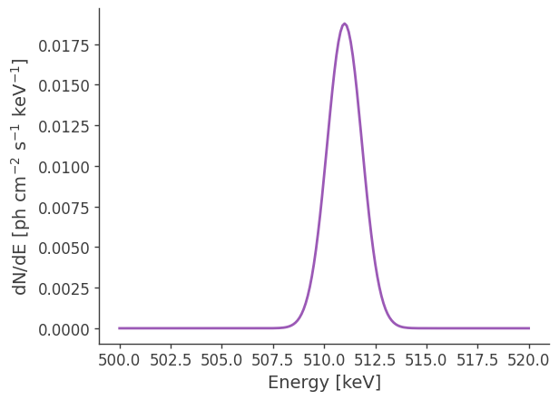
Let’s make some plots to look at the extended source:
[19]:
# Plot spectrum:
energy = np.linspace(500.,520.,201)*u.keV
dnde = src1.spectrum.main.Gaussian(energy)
plt.plot(energy, dnde)
plt.ylabel("dN/dE [$\mathrm{ph \ cm^{-2} \ s^{-1} \ keV^{-1}}$]", fontsize=14)
plt.xlabel("Energy [keV]", fontsize=14)
[19]:
Text(0.5, 0, 'Energy [keV]')
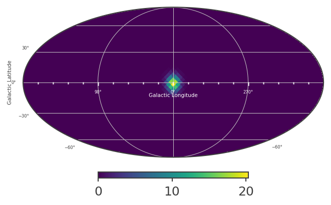
An extended source in astromodels corresponds to a skymap, which is normalized so that the sum over the entire sky, multiplied by the pixel area, equals 1. The pixel values in the skymap serve as weights, which we can use to scale the input spectrum, in order to get the model counts for any location on the sky. This is all handled internally within cosipy, but for demonstration purposes, let’s take a look at the skymap:
[20]:
# Define healpix map matching the detector response:
skymap = HealpixMap(nside = 16, scheme = "ring", dtype = float, coordsys='G')
coords1 = skymap.pix2skycoord(range(skymap.npix))
pix_area = skymap.pixarea().value

# Fill skymap with values from extended source:
skymap[:] = src1.Gaussian_on_sphere(coords1.l.deg, coords1.b.deg)

# Check normalization:
print("summed map: " + str(np.sum(skymap)*pix_area))
summed map: 0.9974653836229357
[21]:
# Plot healpix map:
plot, ax = skymap.plot(ax_kw = {'coord':'G'})
ax.grid()
lon = ax.coords['glon']
lat = ax.coords['glat']
lon.set_axislabel('Galactic Longitude',color='white',fontsize=5)
lat.set_axislabel('Galactic Latitude',fontsize=5)
lon.display_minor_ticks(True)
lat.display_minor_ticks(True)
lon.set_ticks_visible(True)
lon.set_ticklabel_visible(True)
lon.set_ticks(color='white',alpha=0.6)
lat.set_ticks(color='white',alpha=0.6)
lon.set_ticklabel(color='white',fontsize=4)
lat.set_ticklabel(fontsize=4)
lat.set_ticks_visible(True)
lat.set_ticklabel_visible(True)
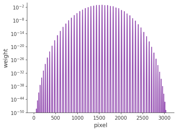
[22]:
# Plot weights directly
# Note: for extended sources the weights also need to include the pixel area.
plt.semilogy(skymap[:]*pix_area)
plt.ylabel("weight")
plt.xlabel("pixel")
plt.ylim(1e-50,1)
[22]:
(1e-50, 1)
Setup the COSI 3ML plugin and perform the likelihood fit
Load the detector response, ori file, and precomputed point source response in Galactic coordinates:
[7]:
#open the orientation file
sc_orientation = SpacecraftHistory.open(data_path+"20280301_3_month_with_orbital_info.ori")

#open the extended source response
dr = ExtendedSourceResponse.open(data_path+"psr_gal_511_DC2.h5")


bkg_dist = {"background":bg_tot.binned_data.project('Em', 'Phi', 'PsiChi')}

# Workaround to avoid inf values. Out bkg should be smooth, but currently it's not.
# Reproduces results before refactoring. It's not _exactly_ the same, since this fudge value was 1e-12, and
# it was added to the expectation, not the normalized bkg
for bckfile in bkg_dist.keys() :
    bkg_dist[bckfile] += sys.float_info.min

#combine the data + the bck like we would get for real data
data = EmCDSBinnedData(gal_511.binned_data.project('Em', 'Phi', 'PsiChi')
                       + bg_tot.binned_data.project('Em', 'Phi', 'PsiChi')
                    )

bkg = FreeNormBinnedBackground(bkg_dist,
                                   sc_history=sc_orientation,
                                   copy = False)

# Currently using the same NnuLambda, Ei and Pol axes as the underlying FullDetectorResponse,
# matching the behavior of v0.3. This is all the current BinnedInstrumentResponse can do.
# In principle, this can be decoupled, and a BinnedInstrumentResponseInterface implementation
# can provide the response for an arbitrary directions, Ei and Pol values.


esr = BinnedThreeMLExtendedSourceResponse(data = data,
                                          precomputed_psr = dr,

                                           polarization_axis = dr.axes['Pol'] if 'Pol' in dr.axes.labels else None,
                                           )

##====


response = BinnedThreeMLModelFolding(data = data, extended_source_response = esr)

like_fun = PoissonLikelihood(data, response, bkg)

cosi = ThreeMLPluginInterface('cosi',
                                  like_fun,
                                  response,
                                  bkg)

cosi.bkg_parameter['background'] = Parameter("background",  # background parameter
                                      1,  # initial value of parameter
                                      unit = u.Hz,
                                      min_value=0,  # minimum value of parameter
                                      max_value=10,  # maximum value of parameter
                                      delta=0.05,  # initial step used by fitting engine
                                      )
WARNING RuntimeWarning: divide by zero encountered in divide
Setup the COSI 3ML plugin:
[8]:
model = Model(src1)  # Model with single source. If we had multiple sources, we would do Model(source1, source2, ...)

# Optional: if you want to call get_log_like manually, then you also need to set the model manually
# 3ML does this internally during the fit though
cosi.set_model(model)


# Gather all plugins and combine with the model in a JointLikelihood object, then perform maximum likelihood fit
plugins = DataList(cosi) # If we had multiple instruments, we would do e.g. DataList(cosi, lat, hawc, ...)

like = JointLikelihood(model, plugins, verbose = False)

like.fit()
17:12:39 INFO set the minimizer to minuit joint_likelihood.py:1017
... Reading Extended source response ...
--> done (source name : gaussian)
WARNING RuntimeWarning: invalid value encountered in log
Best fit values:
| result | unit | |
|---|---|---|
| parameter | ||
| gaussian.spectrum.main.Gaussian.F | (4.6951 +/- 0.0025) x 10^-2 | 1 / (s cm2) |
| background | (2.838 +/- 0.014) x 10^-2 | Hz |
Correlation matrix:
| 1.00 | -0.40 |
| -0.40 | 1.00 |
Values of -log(likelihood) at the minimum:
| -log(likelihood) | |
|---|---|
| cosi | -15275593.788304543 |
| total | -15275593.788304543 |
Values of statistical measures:
| statistical measures | |
|---|---|
| AIC | -30551183.57654398 |
| BIC | -30551163.327751774 |
[8]:
(                                      value  negative_error  positive_error  \
 gaussian.spectrum.main.Gaussian.F  0.046951       -0.000025        0.000025
 background                         0.028381       -0.000140        0.000142

                                       error         unit
 gaussian.spectrum.main.Gaussian.F  0.000025  1 / (s cm2)
 background                         0.000141           Hz  ,
           -log(likelihood)
 cosi   -15275593.788304543
 total  -15275593.788304543)
Perform likelihood fit:
Results
First, let’s just print the results.
[9]:
results = like.results
results.display()

# Print a summary of the optimized model:
print(results.optimized_model["gaussian"])
Best fit values:
| result | unit | |
|---|---|---|
| parameter | ||
| gaussian.spectrum.main.Gaussian.F | (4.6951 +/- 0.0025) x 10^-2 | 1 / (s cm2) |
| background | (2.838 +/- 0.014) x 10^-2 | Hz |
Correlation matrix:
| 1.00 | -0.40 |
| -0.40 | 1.00 |
Values of -log(likelihood) at the minimum:
| -log(likelihood) | |
|---|---|
| cosi | -15275593.788304543 |
| total | -15275593.788304543 |
Values of statistical measures:
| statistical measures | |
|---|---|
| AIC | -30551183.57654398 |
| BIC | -30551163.327751774 |
  * gaussian (extended source):
    * shape:
      * lon0:
        * value: 359.75
        * desc: Longitude of the center of the source
        * min_value: 0.0
        * max_value: 360.0
        * unit: deg
        * is_normalization: false
      * lat0:
        * value: -1.25
        * desc: Latitude of the center of the source
        * min_value: -90.0
        * max_value: 90.0
        * unit: deg
        * is_normalization: false
      * sigma:
        * value: 5.0
        * desc: Standard deviation of the Gaussian distribution
        * min_value: 0.0
        * max_value: 20.0
        * unit: deg
        * is_normalization: false
    * spectrum:
      * main:
        * Gaussian:
          * F:
            * value: 0.04695109527449624
            * desc: Integral between -inf and +inf. Fix this to 1 to obtain a Normal distribution
            * min_value: null
            * max_value: null
            * unit: s-1 cm-2
            * is_normalization: false
          * mu:
            * value: 511.0
            * desc: Central value
            * min_value: null
            * max_value: null
            * unit: keV
            * is_normalization: false
          * sigma:
            * value: 0.85
            * desc: standard deviation
            * min_value: 1.0e-12
            * max_value: null
            * unit: keV
            * is_normalization: false
        * polarization: {}
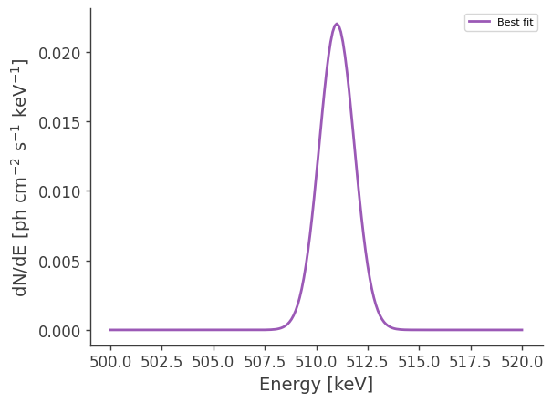
Now let’s make some plots. Let’s first look at the best-fit spectrum:
[10]:
# Best-fit model:
energy = np.linspace(500.,520.,201)*u.keV
flux = results.optimized_model["gaussian"].spectrum.main.shape(energy)

fig,ax = plt.subplots()

ax.plot(energy, flux, label = "Best fit")


plt.ylabel("dN/dE [$\mathrm{ph \ cm^{-2} \ s^{-1} \ keV^{-1}}$]", fontsize=14)
plt.xlabel("Energy [keV]", fontsize=14)
ax.legend()
[10]:
<matplotlib.legend.Legend at 0x7f53c0c99310>
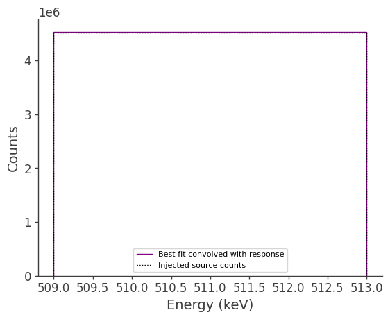
Now let’s compare the predicted counts to the injected counts:
[13]:
# Get expected counts from likelihood scan (i.e. best-fit convolved with response):
#total_expectation = cosi._expected_counts['gaussian']
total_expectation = response.expectation(data)

# Plot:
fig,ax = plt.subplots()

binned_energy_edges = gal_511.binned_data.axes['Em'].edges.value
binned_energy = gal_511.binned_data.axes['Em'].centers.value

ax.stairs(total_expectation.project('Em').todense().contents, binned_energy_edges, color='purple', label = "Best fit convolved with response")
ax.errorbar(binned_energy, total_expectation.project('Em').todense().contents, yerr=np.sqrt(total_expectation.project('Em').todense().contents), color='purple', linewidth=0, elinewidth=1)
ax.stairs(gal_511.binned_data.project('Em').todense().contents, binned_energy_edges, color = 'black', ls = ":", label = "Injected source counts")
ax.errorbar(binned_energy, gal_511.binned_data.project('Em').todense().contents, yerr=np.sqrt(gal_511.binned_data.project('Em').todense().contents), color='black', linewidth=0, elinewidth=1)

ax.set_xlabel("Energy (keV)")
ax.set_ylabel("Counts")

ax.legend()

# Note: We are plotting the error, but it's very small:
print("Error: " +str(np.sqrt(total_expectation.project('Em').todense().contents)))
Error: [2129.0624425]
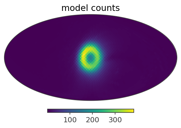
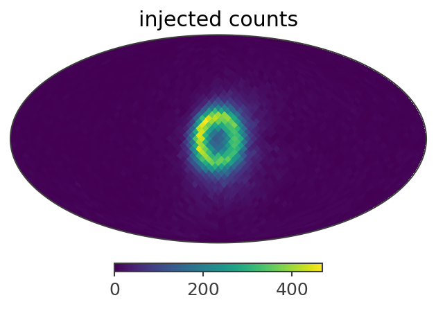
Let’s also compare the projection onto Psichi:
[14]:
# expected src counts:
ax,plot = total_expectation.slice[{'Em':0, 'Phi':5}].project('PsiChi').plot(ax_kw = {'coord':'G'})
plt.title("model counts")

# injected src counts:
ax,plot = gal_511.binned_data.slice[{'Em':0, 'Phi':5}].project('PsiChi').plot(ax_kw = {'coord':'G'})
plt.title("injected counts")
[14]:
Text(0.5, 1.0, 'injected counts')
Here is a summary of the results:
Injected model (extended source): F = 4e-2 ph/cm2/s
Best-fit: F = (4.6951 +/- 0.0025)e-2 ph/cm2/s
We see that the best-fit values are very close to the injected values. The small difference is likely due to the fact that the injected model also has a point source component (which we’ve ignored), having the same specrtum, with a normalization of F = 1e-2 ph/cm2/s. In the next example we’ll see if this point source component can be detected.
**********************************************************
Example 2: Perform Analysis with Two Components
Define the point source. We’ll add this to the model, and keep just the normalization free.
[8]:
# Note: Astromodels only takes ra,dec for point source input:
c = SkyCoord(l=0*u.deg, b=0*u.deg, frame='galactic')
c_icrs = c.transform_to('icrs')

# Define spectrum:
# Note that the units of the Gaussian function below are [F/sigma]=[ph/cm2/s/keV]
F = 1e-2 / u.cm / u.cm / u.s
Fmin = 0 / u.cm / u.cm / u.s
Fmax = 1 / u.cm / u.cm / u.s
mu = 511*u.keV
sigma = 0.85*u.keV
spectrum2 = Gaussian()
spectrum2.F.value = F.value
spectrum2.F.unit = F.unit
spectrum2.F.min_value = Fmin.value
spectrum2.F.max_value = Fmax.value
spectrum2.mu.value = mu.value
spectrum2.mu.unit = mu.unit
spectrum2.sigma.value = sigma.value
spectrum2.sigma.unit = sigma.unit

# Set spectral parameters for fitting:
spectrum2.F.free = True
spectrum2.mu.free = False
spectrum2.sigma.free = False

# Define source:
src2 = PointSource('point_source', ra = c_icrs.ra.deg, dec = c_icrs.dec.deg, spectral_shape=spectrum2)

# Print some info about the source just as a sanity check.
# This will also show you which parameters are free.
print(src2.spectrum.main.shape)

# We can also get a summary of the source info as follows:
#src2.display()
  * description: A Gaussian function
  * formula: $ F \frac{1}{\sigma \sqrt{2 \pi}}\exp{\frac{(x-\mu)^2}{2~(\sigma)^2}} $
  * parameters:
    * F:
      * value: 0.01
      * desc: Integral between -inf and +inf. Fix this to 1 to obtain a Normal distribution
      * min_value: 0.0
      * max_value: 1.0
      * unit: s-1 cm-2
      * is_normalization: false
      * delta: 0.1
      * free: true
    * mu:
      * value: 511.0
      * desc: Central value
      * min_value: null
      * max_value: null
      * unit: keV
      * is_normalization: false
      * delta: 0.1
      * free: false
    * sigma:
      * value: 0.85
      * desc: standard deviation
      * min_value: 1.0e-12
      * max_value: null
      * unit: keV
      * is_normalization: false
      * delta: 0.1
      * free: false
Redefine the first source. We’ll keep just the normalization free.
[9]:
# Define spectrum:
# Note that the units of the Gaussian function below are [F/sigma]=[ph/cm2/s/keV]
F = 4e-2 / u.cm / u.cm / u.s
Fmin = 0 / u.cm / u.cm / u.s
Fmax = 1 / u.cm / u.cm / u.s
mu = 511*u.keV
sigma = 0.85*u.keV
spectrum = Gaussian()
spectrum.F.value = F.value
spectrum.F.unit = F.unit
spectrum.F.min_value = Fmin.value
spectrum.F.max_value = Fmax.value
spectrum.mu.value = mu.value
spectrum.mu.unit = mu.unit
spectrum.sigma.value = sigma.value
spectrum.sigma.unit = sigma.unit

# Set spectral parameters for fitting:
spectrum.F.free = True
spectrum.mu.free = False
spectrum.sigma.free = False

# Define morphology:
morphology = Gaussian_on_sphere(lon0 = 359.75, lat0 = -1.25, sigma = 5)

# Set morphological parameters for fitting:
morphology.lon0.free = False
morphology.lat0.free = False
morphology.sigma.free = False

# Define source:
src1 = ExtendedSource('gaussian', spectral_shape=spectrum, spatial_shape=morphology)

# Print a summary of the source info:
src1.display()

# We can also print the source info as follows.
# This will also show you which parameters are free.
#print(src1.spectrum.main.shape)
#print(src1.spatial_shape)
- gaussian (extended source):
- shape:
- lon0:
- value: 359.75
- desc: Longitude of the center of the source
- min_value: 0.0
- max_value: 360.0
- unit: deg
- is_normalization: False
- lat0:
- value: -1.25
- desc: Latitude of the center of the source
- min_value: -90.0
- max_value: 90.0
- unit: deg
- is_normalization: False
- sigma:
- value: 5.0
- desc: Standard deviation of the Gaussian distribution
- min_value: 0.0
- max_value: 20.0
- unit: deg
- is_normalization: False
- lon0:
- spectrum:
- main:
- Gaussian:
- F:
- value: 0.04
- desc: Integral between -inf and +inf. Fix this to 1 to obtain a Normal distribution
- min_value: 0.0
- max_value: 1.0
- unit: s-1 cm-2
- is_normalization: False
- mu:
- value: 511.0
- desc: Central value
- min_value: None
- max_value: None
- unit: keV
- is_normalization: False
- sigma:
- value: 0.85
- desc: standard deviation
- min_value: 1e-12
- max_value: None
- unit: keV
- is_normalization: False
- F:
- Gaussian:
- main:
- shape:
Setup the COSI 3ML plugin using two sources in the model:
[10]:
%%time


#open the point source response since we also have a point source in this model
pr = FullDetectorResponse.open(data_path+"SMEXv12.511keV.HEALPixO4.binnedimaging.imagingresponse.h5")
instrument_response = BinnedInstrumentResponse(pr,data)

psr = BinnedThreeMLPointSourceResponse(data = data,
                                           instrument_response = instrument_response,
                                           sc_history=sc_orientation,
                                           energy_axis = dr.axes['Ei'],
                                           polarization_axis = dr.axes['Pol'] if 'Pol' in dr.axes.labels else None,
                                           nside = 2*data.axes['PsiChi'].nside)


response = BinnedThreeMLModelFolding(data = data, extended_source_response = esr , point_source_response = psr)

like_fun = PoissonLikelihood(data, response, bkg)

cosi = ThreeMLPluginInterface('cosi',
                                  like_fun,
                                  response,
                                  bkg)

cosi.bkg_parameter['background'] = Parameter("background",  # background parameter
                                      1,  # initial value of parameter
                                      unit = u.Hz,
                                      min_value=0,  # minimum value of parameter
                                      max_value=10,  # maximum value of parameter
                                      delta=0.05,  # initial step used by fitting engine
                                      )


# Add sources to model:
model = Model(src1, src2)  # Model with two sources.
cosi.set_model(model)
CPU times: user 6.03 ms, sys: 224 μs, total: 6.25 ms
Wall time: 14.6 ms
Display the model:
[11]:
esr.axes
[11]:
<histpy.axes.Axes at 0x7fdf2b09d290>
[12]:
psr.axes.ndim
[12]:
3
Before we perform the fit, let’s first change the 3ML console logging level, in order to mimimize the amount of console output.
[13]:
# This is a simple workaround for now to prevent a lot of output.
from threeML import update_logging_level
update_logging_level("CRITICAL")
Perform the likelihood fit:
[14]:
%%time
plugins = DataList(cosi) # If we had multiple instruments, we would do e.g. DataList(cosi, lat, hawc, ...)

like = JointLikelihood(model, plugins, verbose = True)

like.fit()
... Calculating point source response ...
--> done (source name : point_source)
... Reading Extended source response ...
--> done (source name : gaussian)
Best fit values:
| result | unit | |
|---|---|---|
| parameter | ||
| gaussian.spectrum.main.Gaussian.F | (3.196 +/- 0.008) x 10^-2 | 1 / (s cm2) |
| point_source.spectrum.main.Gaussian.F | (1.451 +/- 0.007) x 10^-2 | 1 / (s cm2) |
| background | (3.057 +/- 0.015) x 10^-2 | Hz |
Correlation matrix:
| 1.00 | -0.95 | -0.18 |
| -0.95 | 1.00 | 0.05 |
| -0.18 | 0.05 | 1.00 |
Values of -log(likelihood) at the minimum:
| -log(likelihood) | |
|---|---|
| cosi | -15295331.580454182 |
| total | -15295331.580454182 |
Values of statistical measures:
| statistical measures | |
|---|---|
| AIC | -30590657.160778154 |
| BIC | -30590626.787622396 |
CPU times: user 18.4 s, sys: 279 ms, total: 18.6 s
Wall time: 21.5 s
[14]:
(                                          value  negative_error  \
 gaussian.spectrum.main.Gaussian.F      0.031957       -0.000075
 point_source.spectrum.main.Gaussian.F  0.014508       -0.000074
 background                             0.030573       -0.000150

                                        positive_error     error         unit
 gaussian.spectrum.main.Gaussian.F            0.000079  0.000077  1 / (s cm2)
 point_source.spectrum.main.Gaussian.F        0.000072  0.000073  1 / (s cm2)
 background                                   0.000148  0.000149           Hz  ,
           -log(likelihood)
 cosi   -15295331.580454182
 total  -15295331.580454182)
We see that the normalization of the point source has gone to zero, and we essentially get the same results as the first fit. This is not entirely surprising, considering that the two components have a high degree of degeneracy, and the point source is subdominant.
Note (CK): The injected model may not be exactly the same as the astromodel, because MEGAlib uses a cutoff of the Gaussian spectral distribution at 3 sigma.
*****************************************
Example 3: Working With a Realistic Model
Read in the binned data
We will start with the binned data, since we already learned how to bin data:
[16]:
# background:
bg_tot = BinnedData("Gal_511.yaml")
bg_tot.load_binned_data_from_hdf5(binned_data=data_path+"cosmic_photons_binned_data.hdf5")

# combined data:
data_combined_thin_disk = BinnedData("Gal_511.yaml")
data_combined_thin_disk.load_binned_data_from_hdf5(binned_data=data_path+"combined_binned_data_thin_disk.hdf5")
Define source
This defines a multi-component source with a disk and gaussian component. The disk and bulge components have different spectral characteristics. Spatially, the bulge component is the sum of three different spatial models, with majority of the flux “narrow bulge” with
[17]:
# Spectral Definitions...

models = ["centralPoint","narrowBulge","broadBulge","disk"]

# several lists of parameters for, in order, CentralPoint, NarrowBulge, BroadBulge, and Disk sources
mu         = [511.,511.,511., 511.]*u.keV
sigma      = [0.85,0.85,0.85, 1.27]*u.keV
F          = [0.00012, 0.00028, 0.00073, 1.7e-3]/u.cm/u.cm/u.s
K          = [0.00046, 0.0011, 0.0027, 4.5e-3]/u.cm/u.cm/u.s/u.keV

SpecLine   = [Gaussian(),Gaussian(),Gaussian(),Gaussian()]
SpecOPs    = [SpecFromDat(dat="OPsSpectrum.dat"),SpecFromDat(dat="OPsSpectrum.dat"),SpecFromDat(dat="OPsSpectrum.dat"),SpecFromDat(dat="OPsSpectrum.dat")]

# Set units and fitting parameters; different definition for each spectral model with different norms
for i in range(4):
    SpecLine[i].F.unit = F[i].unit
    SpecLine[i].F.value = F[i].value
    SpecLine[i].F.min_value =0
    SpecLine[i].F.max_value=1
    SpecLine[i].mu.value = mu[i].value
    SpecLine[i].mu.unit = mu[i].unit
    SpecLine[i].sigma.unit = sigma[i].unit
    SpecLine[i].sigma.value = sigma[i].value

    SpecOPs[i].K.value = K[i].value
    SpecOPs[i].K.unit = K[i].unit

    SpecLine[i].sigma.free = False
    SpecLine[i].mu.free = False
    SpecLine[i].F.free = False#True
    SpecOPs[i].K.free = False # not fitting the amplitude of the OPs component for now, since we are only using the 511 response!

SpecLine[-1].F.free = True# actually do fit the flux of the disk component

# Generate Composite Spectra
SpecCentralPoint= SpecLine[0] + SpecOPs[0]
SpecNarrowBulge = SpecLine[1] + SpecOPs[1]
SpecBroadBulge  = SpecLine[2] + SpecOPs[2]
SpecDisk        = SpecLine[3] + SpecOPs[3]
[18]:
# Define Spatial Model Components
MapNarrowBulge = Gaussian_on_sphere(lon0=359.75,lat0=-1.25, sigma = 2.5)
MapBroadBulge = Gaussian_on_sphere(lon0 = 0, lat0 = 0, sigma = 8.7)
MapDisk = Asymm_Gaussian_on_sphere(lon0 = 0, lat0 = 0, a=10, e = 0.99944429,theta=0)
MapDisk.a.max_value = 90
MapDisk.a.value = 90

# Fix fitting parameters (same for all models)
for map in [MapNarrowBulge,MapBroadBulge]:
    map.lon0.free=False
    map.lat0.free=False
    map.sigma.free=False

MapDisk.lon0.free=False
MapDisk.lat0.free=False
MapDisk.a.free=False
MapDisk.e.free=True#False
MapDisk.theta.free=False
For the Asymm_Gaussian_on_sphere model, note that e is the eccentricity of the Gaussian ellipse, defined such that the scale height b of the disk is given by \(b = a \sqrt{(1-e^2)}\)
[19]:
# Define Spatio-spectral models

# Bulge
c = SkyCoord(l=0*u.deg, b=0*u.deg, frame='galactic')
c_icrs = c.transform_to('icrs')
ModelCentralPoint = PointSource('centralPoint', ra = c_icrs.ra.deg, dec = c_icrs.dec.deg, spectral_shape=SpecCentralPoint)
ModelNarrowBulge = ExtendedSource('narrowBulge',spectral_shape=SpecNarrowBulge,spatial_shape=MapNarrowBulge)
ModelBroadBulge = ExtendedSource('broadBulge',spectral_shape=SpecBroadBulge,spatial_shape=MapBroadBulge)

# Disk
ModelDisk = ExtendedSource('disk',spectral_shape=SpecDisk,spatial_shape=MapDisk)
[20]:
ModelDisk
[20]:
- disk (extended source):
- shape:
- lon0:
- value: 0.0
- desc: Longitude of the center of the source
- min_value: 0.0
- max_value: 360.0
- unit: deg
- is_normalization: False
- lat0:
- value: 0.0
- desc: Latitude of the center of the source
- min_value: -90.0
- max_value: 90.0
- unit: deg
- is_normalization: False
- a:
- value: 90.0
- desc: Standard deviation of the Gaussian distribution (major axis)
- min_value: 0.0
- max_value: 90.0
- unit: deg
- is_normalization: False
- e:
- value: 0.99944429
- desc: Excentricity of Gaussian ellipse, e^2 = 1 - (b/a)^2, where b is the standard deviation of the Gaussian distribution (minor axis)
- min_value: 0.0
- max_value: 1.0
- unit:
- is_normalization: False
- theta:
- value: 0.0
- desc: inclination of major axis to a line of constant latitude
- min_value: -90.0
- max_value: 90.0
- unit: deg
- is_normalization: False
- lon0:
- spectrum:
- main:
- composite:
- F_1:
- value: 0.0017
- desc: Integral between -inf and +inf. Fix this to 1 to obtain a Normal distribution
- min_value: 0.0
- max_value: 1.0
- unit: s-1 cm-2
- is_normalization: False
- mu_1:
- value: 511.0
- desc: Central value
- min_value: None
- max_value: None
- unit: keV
- is_normalization: False
- sigma_1:
- value: 1.27
- desc: standard deviation
- min_value: 1e-12
- max_value: None
- unit: keV
- is_normalization: False
- K_2:
- value: 0.0045
- desc: Normalization factor
- min_value: 0.0
- max_value: 1000000.0
- unit: keV-1 s-1 cm-2
- is_normalization: True
- dat_2: OPsSpectrum.dat
- F_1:
- composite:
- main:
- shape:
Make some plots to look at these new extended sources:
[21]:
# Plot spectra at 511 keV
energy = np.linspace(500.,520.,10001)*u.keV
fig, axs = plt.subplots()
for label,m in zip(models,
                   [ModelCentralPoint,ModelNarrowBulge,ModelBroadBulge,ModelDisk]):
    dnde = m.spectrum.main.composite(energy)
    axs.plot(energy, dnde,label=label)

axs.legend()
axs.set_ylabel("dN/dE [$\mathrm{ph \ cm^{-2} \ s^{-1} \ keV^{-1}}$]", fontsize=14)
axs.set_xlabel("Energy [keV]", fontsize=14);
plt.ylim(0,);
#axs[0].set_yscale("log")
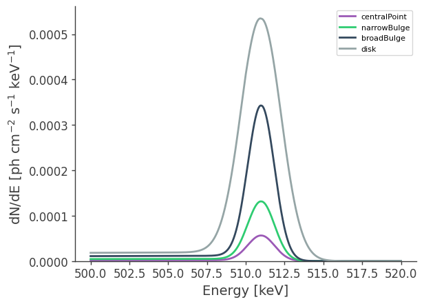
The orthopositronium spectral component appears as the low-energy tail of the 511 keV line.
[22]:
# Define healpix map matching the detector response:
nside_model = 2**4
scheme='ring'
is_nested = (scheme == 'nested')
coordsys='G'

mBroadBulge = HealpixMap(nside = nside_model, scheme = scheme, dtype = float,coordsys=coordsys)
mNarrowBulge = HealpixMap(nside = nside_model, scheme = scheme, dtype = float,coordsys=coordsys)
mPointBulge = HealpixMap(nside = nside_model, scheme = scheme, dtype = float,coordsys=coordsys)
mDisk = HealpixMap(nside = nside_model, scheme=scheme, dtype = float,coordsys=coordsys)

coords = mDisk.pix2skycoord(range(mDisk.npix)) # common among all the galactic maps...

pix_area = mBroadBulge.pixarea().value # common among all the galactic maps with the same pixelization

# Fill skymap with values from extended source:
mNarrowBulge[:] = ModelNarrowBulge.spatial_shape(coords.l.deg, coords.b.deg)
mBroadBulge[:] = ModelBroadBulge.spatial_shape(coords.l.deg, coords.b.deg)
mBulge = mBroadBulge + mNarrowBulge
mDisk[:] = ModelDisk.spatial_shape(coords.l.deg, coords.b.deg)
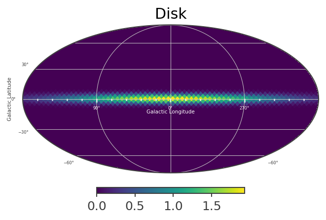
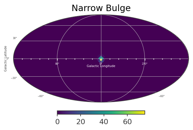
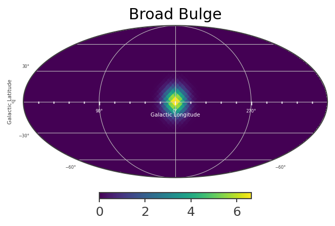
[23]:
List_of_Maps = [mDisk,mNarrowBulge,mBroadBulge]
List_of_Names = ["Disk","Narrow Bulge","Broad Bulge", ]

for n, m in zip(List_of_Names,List_of_Maps):
    plot,ax = m.plot(ax_kw={"coord":"G"})
    ax.grid();
    lon = ax.coords['glon']
    lat = ax.coords['glat']
    lon.set_axislabel('Galactic Longitude',color='white',fontsize=5)
    lat.set_axislabel('Galactic Latitude',fontsize=5)
    lon.display_minor_ticks(True)
    lat.display_minor_ticks(True)
    lon.set_ticks_visible(True)
    lon.set_ticklabel_visible(True)
    lon.set_ticks(color='white',alpha=0.6)
    lat.set_ticks(color='white',alpha=0.6)
    lon.set_ticklabel(color='white',fontsize=4)
    lat.set_ticklabel(fontsize=4)
    lat.set_ticks_visible(True)
    lat.set_ticklabel_visible(True)
    ax.set_title(n)
Instantiate the COSI 3ML plugin and perform the likelihood fit
The following two cells should be run only if not already run in previous examples…
[13]:
# if not previously loaded in example 1, load the response, ori, and psr:

#open the orientation file
sc_orientation = SpacecraftHistory.open(data_path+"20280301_3_month_with_orbital_info.ori")

#open the extended source response
dr = ExtendedSourceResponse.open(data_path+"psr_gal_511_DC2.h5")

#open the point source response
pr = FullDetectorResponse.open(data_path+"SMEXv12.511keV.HEALPixO4.binnedimaging.imagingresponse.h5")
instrument_response = BinnedInstrumentResponse(pr,data)

#setup the bkg model
bkg_dist = {"background":bg_tot.binned_data.project('Em', 'Phi', 'PsiChi')}

# Workaround to avoid inf values. Out bkg should be smooth, but currently it's not.
# Reproduces results before refactoring. It's not _exactly_ the same, since this fudge value was 1e-12, and
# it was added to the expectation, not the normalized bkg
for bckfile in bkg_dist.keys() :
    bkg_dist[bckfile] += sys.float_info.min

bkg = FreeNormBinnedBackground(bkg_dist,
                                   sc_history=sc_orientation,
                                   copy = False)
[24]:
#combine the data + the bck like we would get for real data
data = EmCDSBinnedData(data_combined_thin_disk.binned_data.project('Em', 'Phi', 'PsiChi')
                       + bg_tot.binned_data.project('Em', 'Phi', 'PsiChi')
                    )

esr = BinnedThreeMLExtendedSourceResponse(data = data,
                                          precomputed_psr = dr,

                                           polarization_axis = dr.axes['Pol'] if 'Pol' in dr.axes.labels else None,
                                           )


psr = BinnedThreeMLPointSourceResponse(data = data,
                                           instrument_response = instrument_response,
                                           sc_history=sc_orientation,
                                           energy_axis = dr.axes['Ei'],
                                           polarization_axis = dr.axes['Pol'] if 'Pol' in dr.axes.labels else None,
                                           nside = 2*data.axes['PsiChi'].nside)


response = BinnedThreeMLModelFolding(data = data, extended_source_response = esr , point_source_response = psr)

like_fun = PoissonLikelihood(data, response, bkg)

cosi = ThreeMLPluginInterface('cosi',
                                  like_fun,
                                  response,
                                  bkg)

cosi.bkg_parameter['background'] = Parameter("background",  # background parameter
                                      1,  # initial value of parameter
                                      unit = u.Hz,
                                      min_value=0,  # minimum value of parameter
                                      max_value=10,  # maximum value of parameter
                                      delta=0.05,  # initial step used by fitting engine
                                      )
[25]:
# add sources to thin disk and thick disk models
totalModel =  Model(ModelDisk, ModelBroadBulge,ModelNarrowBulge,ModelCentralPoint)
cosi.set_model(totalModel)
totalModel.display(complete=True)
| N | |
|---|---|
| Point sources | 1 |
| Extended sources | 3 |
| Particle sources | 0 |
Free parameters (2):
| value | min_value | max_value | unit | |
|---|---|---|---|---|
| disk.Wide_Asymm_Gaussian_on_sphere.e | 0.999444 | 0.0 | 1.0 | |
| disk.spectrum.main.composite.F_1 | 0.0017 | 0.0 | 1.0 | s-1 cm-2 |
Fixed parameters (27):
| value | min_value | max_value | unit | |
|---|---|---|---|---|
| disk.Wide_Asymm_Gaussian_on_sphere.lon0 | 0.0 | 0.0 | 360.0 | deg |
| disk.Wide_Asymm_Gaussian_on_sphere.lat0 | 0.0 | -90.0 | 90.0 | deg |
| disk.Wide_Asymm_Gaussian_on_sphere.a | 90.0 | 0.0 | 90.0 | deg |
| disk.Wide_Asymm_Gaussian_on_sphere.theta | 0.0 | -90.0 | 90.0 | deg |
| disk.spectrum.main.composite.mu_1 | 511.0 | None | None | keV |
| disk.spectrum.main.composite.sigma_1 | 1.27 | 0.0 | None | keV |
| disk.spectrum.main.composite.K_2 | 0.0045 | 0.0 | 1000000.0 | keV-1 s-1 cm-2 |
| broadBulge.Gaussian_on_sphere.lon0 | 0.0 | 0.0 | 360.0 | deg |
| broadBulge.Gaussian_on_sphere.lat0 | 0.0 | -90.0 | 90.0 | deg |
| broadBulge.Gaussian_on_sphere.sigma | 8.7 | 0.0 | 20.0 | deg |
| broadBulge.spectrum.main.composite.F_1 | 0.00073 | 0.0 | 1.0 | s-1 cm-2 |
| broadBulge.spectrum.main.composite.mu_1 | 511.0 | None | None | keV |
| broadBulge.spectrum.main.composite.sigma_1 | 0.85 | 0.0 | None | keV |
| broadBulge.spectrum.main.composite.K_2 | 0.0027 | 0.0 | 1000000.0 | keV-1 s-1 cm-2 |
| narrowBulge.Gaussian_on_sphere.lon0 | 359.75 | 0.0 | 360.0 | deg |
| narrowBulge.Gaussian_on_sphere.lat0 | -1.25 | -90.0 | 90.0 | deg |
| narrowBulge.Gaussian_on_sphere.sigma | 2.5 | 0.0 | 20.0 | deg |
| narrowBulge.spectrum.main.composite.F_1 | 0.00028 | 0.0 | 1.0 | s-1 cm-2 |
| narrowBulge.spectrum.main.composite.mu_1 | 511.0 | None | None | keV |
| narrowBulge.spectrum.main.composite.sigma_1 | 0.85 | 0.0 | None | keV |
| narrowBulge.spectrum.main.composite.K_2 | 0.0011 | 0.0 | 1000000.0 | keV-1 s-1 cm-2 |
| centralPoint.position.ra | 266.404988 | 0.0 | 360.0 | deg |
| centralPoint.position.dec | -28.936178 | -90.0 | 90.0 | deg |
| centralPoint.spectrum.main.composite.F_1 | 0.00012 | 0.0 | 1.0 | s-1 cm-2 |
| centralPoint.spectrum.main.composite.mu_1 | 511.0 | None | None | keV |
| centralPoint.spectrum.main.composite.sigma_1 | 0.85 | 0.0 | None | keV |
| centralPoint.spectrum.main.composite.K_2 | 0.00046 | 0.0 | 1000000.0 | keV-1 s-1 cm-2 |
Properties (4):
| value | allowed values | |
|---|---|---|
| disk.spectrum.main.composite.dat_2 | OPsSpectrum.dat | NaN |
| broadBulge.spectrum.main.composite.dat_2 | OPsSpectrum.dat | NaN |
| narrowBulge.spectrum.main.composite.dat_2 | OPsSpectrum.dat | NaN |
| centralPoint.spectrum.main.composite.dat_2 | OPsSpectrum.dat | NaN |
Linked parameters (0):
(none)
Independent variables:
(none)
Linked functions (0):
(none)
Before we perform the fit, let’s first change the 3ML console logging level, in order to mimimize the amount of console output.
[26]:
# This is a simple workaround for now to prevent a lot of output.
from threeML import update_logging_level
update_logging_level("CRITICAL")
[26]:
%%time
# likelihood of data + model
like = JointLikelihood(totalModel, plugins, verbose = True)
like.fit()
... Calculating point source response ...
--> done (source name : centralPoint)
... Reading Extended source response ...
--> done (source name : disk)
... Reading Extended source response ...
--> done (source name : broadBulge)
... Reading Extended source response ...
--> done (source name : narrowBulge)
WARNING RuntimeWarning: divide by zero encountered in log


WARNING RuntimeWarning: invalid value encountered in multiply


WARNING RuntimeWarning: invalid value encountered in multiply


WARNING RuntimeWarning: divide by zero encountered in log


WARNING RuntimeWarning: invalid value encountered in multiply


WARNING RuntimeWarning: invalid value encountered in multiply


WARNING RuntimeWarning: divide by zero encountered in log


WARNING RuntimeWarning: invalid value encountered in multiply


WARNING RuntimeWarning: invalid value encountered in multiply


WARNING RuntimeWarning: divide by zero encountered in log


WARNING RuntimeWarning: invalid value encountered in multiply


WARNING RuntimeWarning: invalid value encountered in multiply


WARNING RuntimeWarning: divide by zero encountered in log


WARNING RuntimeWarning: invalid value encountered in multiply


WARNING RuntimeWarning: invalid value encountered in multiply


WARNING RuntimeWarning: divide by zero encountered in log


WARNING RuntimeWarning: invalid value encountered in multiply


WARNING RuntimeWarning: invalid value encountered in multiply


WARNING RuntimeWarning: divide by zero encountered in log


WARNING RuntimeWarning: invalid value encountered in multiply


WARNING RuntimeWarning: invalid value encountered in multiply


WARNING RuntimeWarning: divide by zero encountered in log


WARNING RuntimeWarning: invalid value encountered in multiply


WARNING RuntimeWarning: invalid value encountered in multiply


WARNING RuntimeWarning: divide by zero encountered in log


WARNING RuntimeWarning: invalid value encountered in multiply


WARNING RuntimeWarning: invalid value encountered in multiply


WARNING RuntimeWarning: divide by zero encountered in log


WARNING RuntimeWarning: invalid value encountered in multiply


WARNING RuntimeWarning: invalid value encountered in multiply


WARNING RuntimeWarning: divide by zero encountered in log


WARNING RuntimeWarning: invalid value encountered in multiply


WARNING RuntimeWarning: invalid value encountered in multiply


WARNING RuntimeWarning: divide by zero encountered in log


WARNING RuntimeWarning: invalid value encountered in multiply


WARNING RuntimeWarning: invalid value encountered in multiply


WARNING RuntimeWarning: divide by zero encountered in log


WARNING RuntimeWarning: invalid value encountered in multiply


WARNING RuntimeWarning: invalid value encountered in multiply


WARNING RuntimeWarning: divide by zero encountered in log


WARNING RuntimeWarning: invalid value encountered in multiply


WARNING RuntimeWarning: invalid value encountered in multiply


WARNING RuntimeWarning: divide by zero encountered in log


WARNING RuntimeWarning: invalid value encountered in multiply


WARNING RuntimeWarning: invalid value encountered in multiply


WARNING RuntimeWarning: divide by zero encountered in log


WARNING RuntimeWarning: invalid value encountered in multiply


WARNING RuntimeWarning: invalid value encountered in multiply


WARNING RuntimeWarning: divide by zero encountered in log


WARNING RuntimeWarning: invalid value encountered in multiply


WARNING RuntimeWarning: invalid value encountered in multiply


WARNING RuntimeWarning: divide by zero encountered in log


WARNING RuntimeWarning: invalid value encountered in multiply


WARNING RuntimeWarning: invalid value encountered in multiply


WARNING RuntimeWarning: divide by zero encountered in log


WARNING RuntimeWarning: invalid value encountered in multiply


WARNING RuntimeWarning: invalid value encountered in multiply


WARNING RuntimeWarning: divide by zero encountered in log


WARNING RuntimeWarning: invalid value encountered in multiply


WARNING RuntimeWarning: invalid value encountered in multiply


WARNING RuntimeWarning: divide by zero encountered in log


WARNING RuntimeWarning: invalid value encountered in multiply


WARNING RuntimeWarning: invalid value encountered in multiply


WARNING RuntimeWarning: divide by zero encountered in log


WARNING RuntimeWarning: invalid value encountered in multiply


WARNING RuntimeWarning: invalid value encountered in multiply


WARNING RuntimeWarning: divide by zero encountered in log


WARNING RuntimeWarning: invalid value encountered in multiply


WARNING RuntimeWarning: invalid value encountered in multiply


WARNING RuntimeWarning: divide by zero encountered in log


WARNING RuntimeWarning: invalid value encountered in multiply


WARNING RuntimeWarning: invalid value encountered in multiply


WARNING RuntimeWarning: divide by zero encountered in log


WARNING RuntimeWarning: invalid value encountered in multiply


WARNING RuntimeWarning: invalid value encountered in multiply


WARNING RuntimeWarning: divide by zero encountered in log


WARNING RuntimeWarning: invalid value encountered in multiply


WARNING RuntimeWarning: invalid value encountered in multiply


WARNING RuntimeWarning: divide by zero encountered in log


WARNING RuntimeWarning: invalid value encountered in multiply


WARNING RuntimeWarning: invalid value encountered in multiply


WARNING RuntimeWarning: divide by zero encountered in log


WARNING RuntimeWarning: invalid value encountered in multiply


WARNING RuntimeWarning: invalid value encountered in multiply


WARNING RuntimeWarning: divide by zero encountered in log


WARNING RuntimeWarning: invalid value encountered in multiply


WARNING RuntimeWarning: invalid value encountered in multiply


WARNING RuntimeWarning: divide by zero encountered in log


WARNING RuntimeWarning: invalid value encountered in multiply


WARNING RuntimeWarning: invalid value encountered in multiply
Best fit values:
| result | unit | |
|---|---|---|
| parameter | ||
| disk.Wide_Asymm_Gaussian_on_sphere.e | (9.99158 +/- 0.00009) x 10^-1 | |
| disk.spectrum.main.composite.F_1 | (6.5291 +/- 0.0031) x 10^-2 | 1 / (s cm2) |
| background | (0 +/- 4) x 10^-9 | Hz |
Correlation matrix:
| 1.00 | -0.06 | 0.00 |
| -0.06 | 1.00 | -0.00 |
| 0.00 | -0.00 | 1.00 |
Values of -log(likelihood) at the minimum:
| -log(likelihood) | |
|---|---|
| cosi | -13327230.78091729 |
| total | -13327230.78091729 |
Values of statistical measures:
| statistical measures | |
|---|---|
| AIC | -26654455.56170437 |
| BIC | -26654425.188548613 |
CPU times: user 46.1 s, sys: 1.55 s, total: 47.6 s
Wall time: 1min 6s
[26]:
(                                             value  negative_error  \
 disk.Wide_Asymm_Gaussian_on_sphere.e  9.991580e-01   -8.876376e-06
 disk.spectrum.main.composite.F_1      6.529095e-02   -3.076891e-05
 background                            1.406895e-12    6.816980e-10

                                       positive_error         error  \
 disk.Wide_Asymm_Gaussian_on_sphere.e    9.160191e-06  9.018284e-06
 disk.spectrum.main.composite.F_1        3.312575e-05  3.194733e-05
 background                              5.072370e-09  2.877034e-09

                                              unit
 disk.Wide_Asymm_Gaussian_on_sphere.e
 disk.spectrum.main.composite.F_1      1 / (s cm2)
 background                                     Hz  ,
          -log(likelihood)
 cosi   -13327230.78091729
 total  -13327230.78091729)
Results
[27]:
# thin disk model to data
results = like.results
results.display()
Best fit values:
| result | unit | |
|---|---|---|
| parameter | ||
| disk.Wide_Asymm_Gaussian_on_sphere.e | (9.99158 +/- 0.00009) x 10^-1 | |
| disk.spectrum.main.composite.F_1 | (6.5291 +/- 0.0031) x 10^-2 | 1 / (s cm2) |
| background | (0 +/- 4) x 10^-9 | Hz |
Correlation matrix:
| 1.00 | -0.06 | 0.00 |
| -0.06 | 1.00 | -0.00 |
| 0.00 | -0.00 | 1.00 |
Values of -log(likelihood) at the minimum:
| -log(likelihood) | |
|---|---|
| cosi | -13327230.78091729 |
| total | -13327230.78091729 |
Values of statistical measures:
| statistical measures | |
|---|---|
| AIC | -26654455.56170437 |
| BIC | -26654425.188548613 |
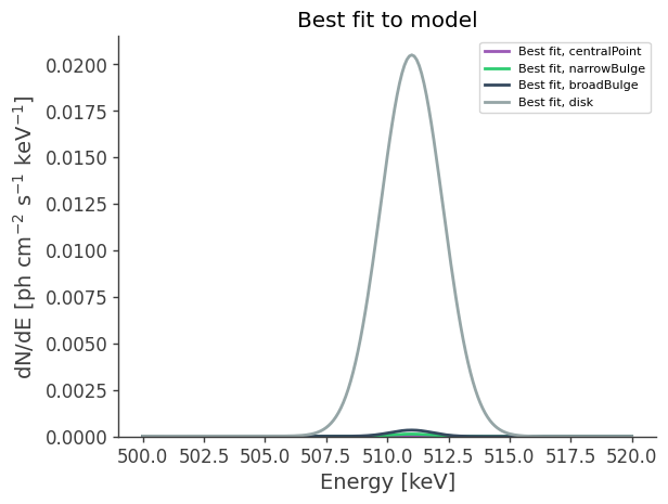
[28]:
# Best-fit model:
energy = np.linspace(500.,520.,201)*u.keV
fluxes = {}

for model in models:
    fluxes[model] = results.optimized_model[model].spectrum.main.shape(energy)

fig,ax = plt.subplots()
for model in models:
    ax.plot(energy, fluxes[model], label = f"Best fit, {model}",ls='-')
ax.set_ylabel("dN/dE [$\mathrm{ph \ cm^{-2} \ s^{-1} \ keV^{-1}}$]", fontsize=14)
ax.set_xlabel("Energy [keV]", fontsize=14)
ax.set_title("Best fit to model")
ax.legend()
ax.set_ylim(0,);