Spectral fitting example (GRB)
To run this, you need the following files, which can be downloaded using the first few cells of this notebook:
orientation file (20280301_3_month_with_orbital_info.fits)
binned data (grb_binned_data.hdf5 & bkg_binned_data_1s_local.hdf5)
detector response (SMEXv12.Continuum.HEALPixO3_10bins_log_flat.binnedimaging.imagingresponse.h5)
The binned data are simulations of GRB090206620 and albedo photon background produced using the COSI SMEX mass model. The detector response needs to be unzipped before running the notebook.
This notebook fits the spectrum of a GRB simulated using MEGAlib and combined with background.
3ML is a high-level interface that allows multiple datasets from different instruments to be used coherently to fit the parameters of source model. A source model typically consists of a list of sources with parametrized spectral shapes, sky locations and, for extended sources, shape. Polarization is also possible. A “coherent” analysis, in this context, means that the source model parameters are fitted using all available datasets simultanously, rather than performing individual fits and finding a well-suited common model a posteriori.
In order for a dataset to be included in 3ML, each instrument needs to provide a “plugin”. Each plugin is responsible for reading the data, convolving the source model (provided by 3ML) with the instrument response, and returning a likelihood. In our case, we’ll compute a binned Poisson likelihood:
where \(d_i\) are the counts on each bin and \(\lambda_i\) are the expected counts given a source model with parameters \(\mathbf{x}\).
In this example, we will fit a single point source with a known location. We’ll assume the background is known and fixed up to a scaling factor. Finally, we will fit a Band function:
where \(K\) (normalization), \(\alpha\) & \(\beta\) (spectral indeces), and \(x_p\) (peak energy) are the free parameters, while \(E_{piv}\) is the pivot energy which is fixed (and arbitrary).
Considering these assumptions:
where \(B*b_i\) are the estimated counts due to background in each bin of the Compton data space with \(B\) the amplitude and \(b_i\) the shape of the background, and \(s_i\) are the corresponding expected counts from the source, the goal is then to find the values of \(\mathbf{x} = [K, \alpha, \beta, x_p]\) and \(B\) that maximize \(\mathcal{L}\). These are the best estimations of the parameters.
The final module needs to also fit the time-dependent background, handle multiple point-like and extended sources, as well as all the spectral models supported by 3ML. Eventually, it will also fit the polarization angle. However, this simple example already contains all the necessary pieces to do a fit.
[1]:
from cosipy import BinnedData
from cosipy.spacecraftfile import SpacecraftHistory
from cosipy.response.FullDetectorResponse import FullDetectorResponse
from cosipy.util import fetch_wasabi_file

from cosipy.statistics import PoissonLikelihood
from cosipy.background_estimation import FreeNormBinnedBackground
from cosipy.interfaces import ThreeMLPluginInterface
from cosipy.response import BinnedThreeMLModelFolding, BinnedInstrumentResponse, BinnedThreeMLPointSourceResponse
from cosipy.data_io import EmCDSBinnedData

import sys

import astropy.units as u
from astropy.time import Time
from astropy.stats import poisson_conf_interval

import numpy as np
import matplotlib.pyplot as plt

from threeML import Band, PointSource, Model, JointLikelihood, DataList
from astromodels import Parameter, Powerlaw

from pathlib import Path

%matplotlib inline
14:46:32 WARNING   The naima package is not available. Models that depend on it will not be         functions.py:43
                  available
         WARNING   The GSL library or the pygsl wrapper cannot be loaded. Models that depend on it  functions.py:65
                  will not be available.
14:46:33 WARNING   The ebltable package is not available. Models that depend on it will not be     absorption.py:33
                  available
14:46:33 INFO Starting 3ML! __init__.py:44
WARNING WARNINGs here are NOT errors __init__.py:45
WARNING but are inform you about optional packages that can be installed __init__.py:46
WARNING to disable these messages, turn off start_warning in your config file __init__.py:47
WARNING ROOT minimizer not available minimization.py:1208
WARNING Multinest minimizer not available minimization.py:1218
WARNING PyGMO is not available minimization.py:1228
         WARNING   The cthreeML package is not installed. You will not be able to use plugins which  __init__.py:95
                  require the C/C++ interface (currently HAWC)
         WARNING   Could not import plugin FermiLATLike.py. Do you have the relative instrument     __init__.py:136
                  software installed and configured?
         WARNING   Could not import plugin HAWCLike.py. Do you have the relative instrument         __init__.py:136
                  software installed and configured?
WARNING No fermitools installed lat_transient_builder.py:44
         WARNING   Env. variable OMP_NUM_THREADS is not set. Please set it to 1 for optimal         __init__.py:345
                  performances in 3ML
         WARNING   Env. variable MKL_NUM_THREADS is not set. Please set it to 1 for optimal         __init__.py:345
                  performances in 3ML
         WARNING   Env. variable NUMEXPR_NUM_THREADS is not set. Please set it to 1 for optimal     __init__.py:345
                  performances in 3ML
Download and read in binned data
Define the path to the directory containing the data, detector response, orientation file, and yaml files if they have already been downloaded, or the directory to download the files into
[2]:
data_path = Path("") # /path/to/files. Current dir by default
Download the orientation file (684.38 MB)
[3]:
fetch_wasabi_file('COSI-SMEX/develop/Data/Orientation/20280301_3_month_with_orbital_info.fits', output=str(data_path / '20280301_3_month_with_orbital_info.fits'), checksum = '5e69bc1d55fab9390f90635690f62896')
A file named 20280301_3_month_with_orbital_info.fits already exists with the specified checksum (5e69bc1d55fab9390f90635690f62896). Skipping.
Download the binned GRB data (76.90 KB)
[4]:
fetch_wasabi_file('COSI-SMEX/cosipy_tutorials/grb_spectral_fit_local_frame/grb_binned_data.hdf5', output=str(data_path / 'grb_binned_data.hdf5'), checksum = 'fcf7022369b6fb378d67b780fc4b5db8')
A file named grb_binned_data.hdf5 already exists with the specified checksum (fcf7022369b6fb378d67b780fc4b5db8). Skipping.
Download the binned background data (255.97 MB)
[5]:
fetch_wasabi_file('COSI-SMEX/cosipy_tutorials/grb_spectral_fit_local_frame/bkg_binned_data_1s_local.hdf5', output=str(data_path / 'bkg_binned_data_1s_local.hdf5'), checksum = 'b842a7444e6fc1a5dd567b395c36ae7f')
A file named bkg_binned_data_1s_local.hdf5 already exists with the specified checksum (b842a7444e6fc1a5dd567b395c36ae7f). Skipping.
Download the response file (596.06 MB)
[6]:
fetch_wasabi_file('COSI-SMEX/develop/Data/Responses/SMEXv12.Continuum.HEALPixO3_10bins_log_flat.binnedimaging.imagingresponse.h5', output=str(data_path / 'SMEXv12.Continuum.HEALPixO3_10bins_log_flat.binnedimaging.imagingresponse.h5'), checksum = 'eb72400a1279325e9404110f909c7785')
A file named SMEXv12.Continuum.HEALPixO3_10bins_log_flat.binnedimaging.imagingresponse.h5 already exists with the specified checksum (eb72400a1279325e9404110f909c7785). Skipping.
Read in the spacecraft orientation file & select the beginning and end times of the GRB
[7]:
tmin = Time(1842597410.0, format='unix')
tmax = Time(1842597450.0, format='unix')
sc_orientation = SpacecraftHistory.open(data_path / "20280301_3_month_with_orbital_info.fits", tmin, tmax)
sc_orientation = sc_orientation.select_interval(tmin, tmax) # Function changed name during refactoring
Create BinnedData objects for the GRB only and background only. The GRB only simulation is not used for the spectral fit, but can be used to compare the fitted spectrum to the source simulation
[8]:
grb = BinnedData(data_path / "grb.yaml")
bkg = BinnedData(data_path / "background.yaml")
Load binned .hdf5 files
[9]:
grb.load_binned_data_from_hdf5(binned_data=data_path / "grb_binned_data.hdf5")
bkg.load_binned_data_from_hdf5(binned_data=data_path / "bkg_binned_data_1s_local.hdf5")
Define the path to the detector response
[10]:
dr_path = data_path / "SMEXv12.Continuum.HEALPixO3_10bins_log_flat.binnedimaging.imagingresponse.h5"  # path to detector response
fetch_wasabi_file(
    'COSI-SMEX/develop/Data/Responses/SMEXv12.Continuum.HEALPixO3_10bins_log_flat.binnedimaging.imagingresponse.h5',
    output=str(dr_path),
    checksum='eb72400a1279325e9404110f909c7785')

dr = FullDetectorResponse.open(dr_path)
A file named SMEXv12.Continuum.HEALPixO3_10bins_log_flat.binnedimaging.imagingresponse.h5 already exists with the specified checksum (eb72400a1279325e9404110f909c7785). Skipping.
Perform spectral fit
Define time window of binned background simulation to use for background model
[11]:
bkg_tmin = 1842597310.0
bkg_tmax = 1842597550.0
bkg_min = np.where(bkg.binned_data.axes['Time'].edges.value == bkg_tmin)[0][0]
bkg_max = np.where(bkg.binned_data.axes['Time'].edges.value == bkg_tmax)[0][0]
bkg_dist = bkg.binned_data.slice[{'Time': slice(bkg_min, bkg_max)}].project('Em', 'Phi', 'PsiChi')

# Workaround to avoid inf values. Out bkg should be smooth, but currently it's not.
# Reproduces results before refactoring. It's not _exactly_ the same, since this fudge value was 1e-12, and
# it was added to the expectation, not the normalized bkg
bkg_dist += sys.float_info.min
Find the overlap between binned background simulation and the grb signal
[12]:
bkg_overlap_tmin = 1842597410.0
bkg_overlap_tmax = 1842597450.0

bkg_overlap_min, bkg_overlap_max = np.searchsorted(bkg.binned_data.axes['Time'].edges.value,
                                   (bkg_overlap_tmin, bkg_overlap_tmax), side='left')

bkg_overlap = bkg.binned_data.slice[{'Time': slice(bkg_overlap_min, bkg_overlap_max)}]
Set background parameter, which is used to fit the amplitude of the background, and instantiate the COSI 3ML plugin
[13]:
# Wrap the raw BinnedData objects into the appropiate data interface.
data = EmCDSBinnedData(grb.binned_data.project('Em', 'Phi', 'PsiChi') + bkg_overlap.project('Em', 'Phi', 'PsiChi'))

# Use the background model to initialize a background expectation interface.
# For this particular background interface implementation, only the normalization values are free.
bkg_model = FreeNormBinnedBackground(bkg_dist,
                               sc_history=sc_orientation,
                               copy = False)

instrument_response = BinnedInstrumentResponse(dr, data)

# Currently using the same NnuLambda, Ei and Pol axes as the underlying FullDetectorResponse,
# matching the behavior of v0.3. This is all the current BinnedInstrumentResponse can do.
# In principle, this can be decoupled, and a BinnedInstrumentResponseInterface implementation
# can provide the response for an arbitrary directions, Ei and Pol values.
# NOTE: this is currently only implemented for data in local coords
psr = BinnedThreeMLPointSourceResponse(data = data,
                                        instrument_response = instrument_response,
                                        sc_history=sc_orientation,
                                        energy_axis = dr.axes['Ei'],
                                        polarization_axis = dr.axes['Pol'] if 'Pol' in dr.axes.labels else None,
                                        nside = 2*data.axes['PsiChi'].nside)

response = BinnedThreeMLModelFolding(data = data, point_source_response = psr)

like_fun = PoissonLikelihood(data, response, bkg_model)

cosi = ThreeMLPluginInterface('cosi',
                                like_fun,
                                response,
                                bkg_model)

# Nuisance parameter guess, bounds, etc.
cosi.bkg_parameter['bkg_norm'] = Parameter("bkg_norm",  # background parameter
                                    1,
                                    unit  = u.Hz,# initial value of parameter
                                    min_value=0,  # minimum value of parameter
                                    max_value=5,  # maximum value of parameter
                                    delta=1e-3,  # initial step used by fitting engine
                                    )
Define a point source at the known location with a Band function spectrum and add it to the model
[14]:
# Set model to fit
l = 93.
b = -53.

alpha = -1
beta = -3
xp = 450. * u.keV
piv = 500. * u.keV
K = 1 / u.cm / u.cm / u.s / u.keV

spectrum = Band()
spectrum.beta.min_value = -15.0
spectrum.alpha.value = alpha
spectrum.beta.value = beta
spectrum.xp.value = xp.value
spectrum.K.value = K.value
spectrum.piv.value = piv.value
spectrum.xp.unit = xp.unit
spectrum.K.unit = K.unit
spectrum.piv.unit = piv.unit

source = PointSource("source",  # Name of source (arbitrary, but needs to be unique)
                        l=l,  # Longitude (deg)
                        b=b,  # Latitude (deg)
                        spectral_shape=spectrum)  # Spectral model

model = Model(source)                              # Model with single source. If we had multiple sources, we would do Model(source1, source2, ...)
Gather all plugins and combine with the model in a JointLikelihood object, then perform maximum likelihood fit
[15]:
%%time

plugins = DataList(cosi) # If we had multiple instruments, we would do e.g. DataList(cosi, lat, hawc, ...)

like = JointLikelihood(model, plugins, verbose = False)

_ = like.fit()
14:46:50 INFO set the minimizer to minuit joint_likelihood.py:994
14:47:58 WARNING   50.94 percent of samples have been thrown away because they failed the  analysis_results.py:1645
                  constraints on the parameters. This results might not be suitable for
                  error propagation. Enlarge the boundaries until you loose less than 1
                  percent of the samples.
Best fit values:
| result | unit | |
|---|---|---|
| parameter | ||
| source.spectrum.main.Band.K | (3.08 -0.20 +0.21) x 10^-2 | 1 / (keV s cm2) |
| source.spectrum.main.Band.alpha | (-2.8 +/- 0.5) x 10^-1 | |
| source.spectrum.main.Band.xp | (4.76 +/- 0.05) x 10^2 | keV |
| source.spectrum.main.Band.beta | -6.8 +/- 1.2 | |
| bkg_norm | 5.000000 +/- 0.000010 | Hz |
Correlation matrix:
| 1.00 | 0.97 | -0.37 | 0.19 | 0.00 |
| 0.97 | 1.00 | -0.16 | 0.17 | 0.00 |
| -0.37 | -0.16 | 1.00 | -0.17 | -0.00 |
| 0.19 | 0.17 | -0.17 | 1.00 | 0.00 |
| 0.00 | 0.00 | -0.00 | 0.00 | 1.00 |
Values of -log(likelihood) at the minimum:
| -log(likelihood) | |
|---|---|
| cosi | 42873.90843683667 |
| total | 42873.90843683667 |
Values of statistical measures:
| statistical measures | |
|---|---|
| AIC | 85757.81709069194 |
| BIC | 85810.46634249632 |
CPU times: user 24min 47s, sys: 1.35 s, total: 24min 48s
Wall time: 1min 7s
Error propagation and plotting
Define Band function spectrum injected into MEGAlib
[16]:
alpha_inj = -0.360
beta_inj = -11.921
E0_inj = 288.016 * u.keV
xp_inj = E0_inj * (alpha_inj + 2)
piv_inj = 1. * u.keV
K_inj = 0.283 / u.cm / u.cm / u.s / u.keV

spectrum_inj = Band()

spectrum_inj.beta.min_value = -15.0

spectrum_inj.alpha.value = alpha_inj
spectrum_inj.beta.value = beta_inj
spectrum_inj.xp.value = xp_inj.value
spectrum_inj.K.value = K_inj.value
spectrum_inj.piv.value = piv_inj.value

spectrum_inj.xp.unit = xp_inj.unit
spectrum_inj.K.unit = K_inj.unit
spectrum_inj.piv.unit = piv_inj.unit
The summary of the results above tell you the optimal values of the parameters, as well as the errors. Propogate the errors to the “evaluate_at” method of the spectrum
[17]:
results = like.results

print(results.display())

parameters = {par.name:results.get_variates(par.path)
              for par in results.optimized_model["source"].parameters.values()
              if par.free}

results_err = results.propagate(results.optimized_model["source"].spectrum.main.shape.evaluate_at, **parameters)

print(results.optimized_model["source"])
Best fit values:
| result | unit | |
|---|---|---|
| parameter | ||
| source.spectrum.main.Band.K | (3.08 -0.20 +0.21) x 10^-2 | 1 / (keV s cm2) |
| source.spectrum.main.Band.alpha | (-2.8 +/- 0.5) x 10^-1 | |
| source.spectrum.main.Band.xp | (4.76 +/- 0.05) x 10^2 | keV |
| source.spectrum.main.Band.beta | -6.8 +/- 1.2 | |
| bkg_norm | 5.000000 +/- 0.000010 | Hz |
Correlation matrix:
| 1.00 | 0.97 | -0.37 | 0.19 | 0.00 |
| 0.97 | 1.00 | -0.16 | 0.17 | 0.00 |
| -0.37 | -0.16 | 1.00 | -0.17 | -0.00 |
| 0.19 | 0.17 | -0.17 | 1.00 | 0.00 |
| 0.00 | 0.00 | -0.00 | 0.00 | 1.00 |
Values of -log(likelihood) at the minimum:
| -log(likelihood) | |
|---|---|
| cosi | 42873.90843683667 |
| total | 42873.90843683667 |
Values of statistical measures:
| statistical measures | |
|---|---|
| AIC | 85757.81709069194 |
| BIC | 85810.46634249632 |
None
  * source (point source):
    * position:
      * l:
        * value: 93.0
        * desc: Galactic longitude
        * min_value: 0.0
        * max_value: 360.0
        * unit: deg
        * is_normalization: false
      * b:
        * value: -53.0
        * desc: Galactic latitude
        * min_value: -90.0
        * max_value: 90.0
        * unit: deg
        * is_normalization: false
      * equinox: J2000
    * spectrum:
      * main:
        * Band:
          * K:
            * value: 0.03075834274428146
            * desc: Differential flux at the pivot energy
            * min_value: 1.0e-50
            * max_value: null
            * unit: keV-1 s-1 cm-2
            * is_normalization: true
          * alpha:
            * value: -0.2772934236796841
            * desc: low-energy photon index
            * min_value: -1.5
            * max_value: 3.0
            * unit: ''
            * is_normalization: false
          * xp:
            * value: 475.55032499581745
            * desc: peak in the x * x * N (nuFnu if x is a energy)
            * min_value: 10.0
            * max_value: null
            * unit: keV
            * is_normalization: false
          * beta:
            * value: -6.787918153546224
            * desc: high-energy photon index
            * min_value: -15.0
            * max_value: -1.6
            * unit: ''
            * is_normalization: false
          * piv:
            * value: 500.0
            * desc: pivot energy
            * min_value: null
            * max_value: null
            * unit: keV
            * is_normalization: false
        * polarization: {}
Evaluate the flux and errors at a range of energies for the fitted and injected spectra, and the simulated source flux
[18]:
energy = np.geomspace(100*u.keV,10*u.MeV).to_value(u.keV)

flux_lo = np.zeros_like(energy)
flux_median = np.zeros_like(energy)
flux_hi = np.zeros_like(energy)
flux_inj = np.zeros_like(energy)

for i, e in enumerate(energy):
    flux = results_err(e)
    flux_median[i] = flux.median
    flux_lo[i], flux_hi[i] = flux.equal_tail_interval(cl=0.68)
    flux_inj[i] = spectrum_inj.evaluate_at(e)

binned_energy_edges = grb.binned_data.axes['Em'].edges.value
binned_energy = np.array([])
bin_sizes = np.array([])

for i in range(len(binned_energy_edges)-1):
    binned_energy = np.append(binned_energy, (binned_energy_edges[i+1] + binned_energy_edges[i]) / 2)
    bin_sizes = np.append(bin_sizes, binned_energy_edges[i+1] - binned_energy_edges[i])

expectation = response.expectation()
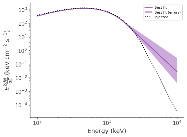
Plot the fitted and injected spectra
[19]:
fig,ax = plt.subplots()

ax.plot(energy, energy*energy*flux_median, label = "Best fit")
ax.fill_between(energy, energy*energy*flux_lo, energy*energy*flux_hi, alpha = .5, label = "Best fit (errors)")
ax.plot(energy, energy*energy*flux_inj, color = 'black', ls = ":", label = "Injected")

ax.set_xscale("log")
ax.set_yscale("log")

ax.set_xlabel("Energy (keV)")
ax.set_ylabel(r"$E^2 \frac{dN}{dE}$ (keV cm$^{-2}$ s$^{-1}$)")

_ = ax.legend()
[20]:
def compute_errors(counts):
    gaussian_error = np.zeros(len(counts))
    poisson_error  = np.zeros((2, len(counts)))

    hi_mask = (counts > 5)
    gaussian_error[hi_mask] = np.sqrt(counts[hi_mask])
    poisson_error[:,~hi_mask] = poisson_conf_interval(counts[~hi_mask], interval="frequentist-confidence", sigma=1)

    return gaussian_error, poisson_error
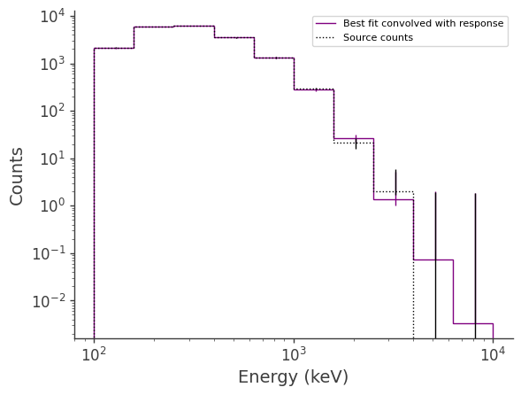
Plot the fitted spectrum convolved with the response, as well as the simulated source counts
[21]:
em_inj = grb.binned_data.project('Em').todense().contents
em_fit = expectation.project('Em').todense().contents

fit_gaussian_error, fit_poisson_error = compute_errors(em_fit)
inj_gaussian_error, inj_poisson_error = compute_errors(em_inj)

fig,ax = plt.subplots()

ax.stairs(expectation.project('Em').todense().contents, binned_energy_edges, color='purple', label = "Best fit convolved with response")
ax.errorbar(binned_energy, expectation.project('Em').todense().contents, yerr=fit_poisson_error, color='purple', linewidth=0, elinewidth=1)
ax.errorbar(binned_energy, expectation.project('Em').todense().contents, yerr=fit_gaussian_error, color='purple', linewidth=0, elinewidth=1)
ax.stairs(grb.binned_data.project('Em').todense().contents, binned_energy_edges, color = 'black', ls = ":", label = "Source counts")
ax.errorbar(binned_energy, grb.binned_data.project('Em').todense().contents, yerr=fit_poisson_error, color='black', linewidth=0, elinewidth=1)
ax.errorbar(binned_energy, grb.binned_data.project('Em').todense().contents, yerr=fit_gaussian_error, color='black', linewidth=0, elinewidth=1)

ax.set_xscale("log")
ax.set_yscale("log")

ax.set_xlabel("Energy (keV)")
ax.set_ylabel("Counts")

_ = ax.legend()
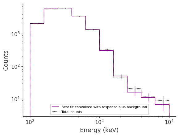
Plot the fitted spectrum convolved with the response plus the fitted background, as well as the simulated source+background counts
[22]:
expectation_bkg = bkg_model.expectation(copy = True)

fit_bkg_gaussian_error, fit_bkg_poisson_error = compute_errors(expectation.project('Em').todense().contents + expectation_bkg.project('Em').todense().contents)
inj_bkg_gaussian_error, inj_bkg_poisson_error = compute_errors(data.data.project('Em').todense().contents)

fig,ax = plt.subplots()
ax.stairs(expectation.project('Em').todense().contents + expectation_bkg.project('Em').todense().contents, binned_energy_edges, color='purple', label = "Best fit convolved with response plus background")
ax.errorbar(binned_energy, expectation.project('Em').todense().contents+expectation_bkg.project('Em').todense().contents, yerr=fit_bkg_poisson_error, color='purple', linewidth=0, elinewidth=1)
ax.errorbar(binned_energy, expectation.project('Em').todense().contents+expectation_bkg.project('Em').todense().contents, yerr=fit_bkg_gaussian_error, color='purple', linewidth=0, elinewidth=1)
ax.stairs(data.data.project('Em').todense().contents, binned_energy_edges, color = 'black', ls = ":", label = "Total counts")
ax.errorbar(binned_energy, data.data.project('Em').todense().contents, yerr=inj_bkg_poisson_error, color='black', linewidth=0, elinewidth=1)
ax.errorbar(binned_energy, data.data.project('Em').todense().contents, yerr=inj_bkg_gaussian_error, color='black', linewidth=0, elinewidth=1)


ax.set_xscale("log")
ax.set_yscale("log")

ax.set_xlabel("Energy (keV)")
ax.set_ylabel("Counts")

ax.legend()

plt.show()